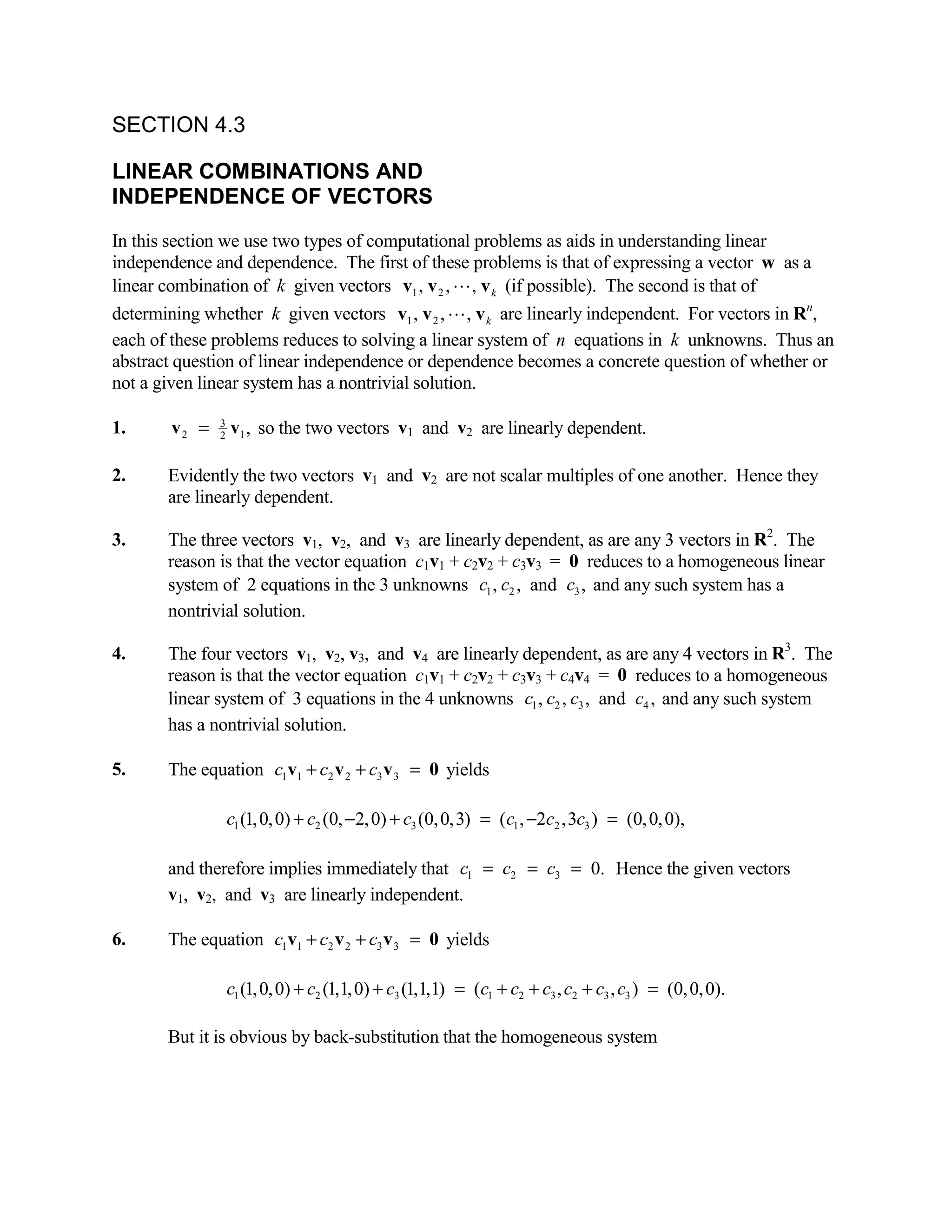
This section discusses linear combinations and independence of vectors. It explains that determining if vectors are linearly dependent or independent involves solving a linear system of equations. The document then provides examples of checking if sets of vectors are linearly dependent or independent by setting up and row reducing the associated coefficient matrix. It demonstrates that the reduced row echelon form reveals whether a nontrivial solution exists, indicating dependence or independence.

1. SECTION 4.3
LINEAR COMBINATIONS AND
INDEPENDENCE OF VECTORS
In this section we use two types of computational problems as aids in understanding linear
independence and dependence. The first of these problems is that of expressing a vector w as a
linear combination of k given vectors v1 , v 2 , , v k (if possible). The second is that of
determining whether k given vectors v1 , v 2 , , v k are linearly independent. For vectors in Rn,
each of these problems reduces to solving a linear system of n equations in k unknowns. Thus an
abstract question of linear independence or dependence becomes a concrete question of whether or
not a given linear system has a nontrivial solution.
1. v2 = 3
2
v1 , so the two vectors v1 and v2 are linearly dependent.
2. Evidently the two vectors v1 and v2 are not scalar multiples of one another. Hence they
are linearly dependent.
3. The three vectors v1, v2, and v3 are linearly dependent, as are any 3 vectors in R2. The
reason is that the vector equation c1v1 + c2v2 + c3v3 = 0 reduces to a homogeneous linear
system of 2 equations in the 3 unknowns c1 , c2 , and c3 , and any such system has a
nontrivial solution.
4. The four vectors v1, v2, v3, and v4 are linearly dependent, as are any 4 vectors in R3. The
reason is that the vector equation c1v1 + c2v2 + c3v3 + c4v4 = 0 reduces to a homogeneous
linear system of 3 equations in the 4 unknowns c1 , c2 , c3 , and c4 , and any such system
has a nontrivial solution.
5. The equation c1 v1 + c2 v 2 + c3 v 3 = 0 yields
c1 (1, 0, 0) + c2 (0, −2, 0) + c3 (0, 0,3) = (c1 , −2c2 ,3c3 ) = (0, 0, 0),
and therefore implies immediately that c1 = c2 = c3 = 0. Hence the given vectors
v1, v2, and v3 are linearly independent.
6. The equation c1 v1 + c2 v 2 + c3 v 3 = 0 yields
c1 (1, 0, 0) + c2 (1,1, 0) + c3 (1,1,1) = (c1 + c2 + c3 , c2 + c3 , c3 ) = (0, 0, 0).
But it is obvious by back-substitution that the homogeneous system

2. c1 + c2 + c3 = 0
c2 + c3 = 0
c3 = 0
has only the trivial solution c1 = c2 = c3 = 0. Hence the given vectors
v1, v2, and v3 are linearly independent.
7. The equation c1 v1 + c2 v 2 + c3 v 3 = 0 yields
c1 (2,1, 0, 0) + c2 (3, 0,1, 0) + c3 (4, 0, 0,1) = (2c1 + 3c2 , c1 , c2 , c3 ) = (0, 0, 0, 0).
Obviously it follows immediately that c1 = c2 = c3 = 0. Hence the given vectors
v1, v2, and v3 are linearly independent.
8. Here inspection of the three given vectors reveals that v 3 = v1 + v 2 , so the vectors
v1, v2, and v3 are linearly dependent.
In Problems 9-16 we first set up the linear system to be solved for the linear combination
coefficients {ci }, and then show the reduction of its augmented coefficient matrix A to reduced
echelon form E.
9. c1 v1 + c2 v 2 = w
5 3 1  1 0 2 
A =  3 2 0  → 0 1 −3 = E
   
 4 5 −7 
  0 0 0 
 
We see that the system of 3 equations in 2 unknowns has the unique solution
c1 = 2, c2 = −3, so w = 2 v1 − 3v 2 .
10. c1 v1 + c2 v 2 = w
 −3 6 3  1 0 7 
 1 −2 −1 → 0 1 4  = E
A =    
 −2 3 −2 
  0 0 0 
 
We see that the system of 3 equations in 2 unknowns has the unique solution
c1 = 7, c2 = 4, so w = 7 v1 + 4 v 2 .

3. 11. c1 v1 + c2 v 2 = w
7 3 1 1 0 1 
 −6 −3 0   
A =   →  0 1 −2  = E
4 2 0 0 0 0 
   
 5 3 −1 0 0 0 
We see that the system of 4 equations in 2 unknowns has the unique solution
c1 = 1, c2 = −2, so w = v1 − 2 v 2 .
12. c1 v1 + c2 v 2 = w
 7 −2 4  1 0 2
 3 −2 −4   5
A =   → 0 1  = E
 −1 1 3 0 0 0
   
 9 −3 3  0 0 0
We see that the system of 4 equations in 2 unknowns has the unique solution
c1 = 2, c2 = 5, so w = 2 v1 + 5v 2 .
13. c1 v1 + c2 v 2 = w
1 5 5 1 0 0
A =  5 −3 2  → 0 1 0  = E
   
 −3 4 −2 
  0 0 1 
 
The last row of E corresponds to the scalar equation 0c1 + 0c2 = 1, so the system of 3
equations in 2 unknowns is inconsistent. This means that w cannot be expressed as a
linear combination of v1 and v2.
14. c1v1 + c2 v 2 + c3 v 3 = w
1 0 0 2  1 0 0 0
 0 1 − 1 − 3  0
A =   → 0 1 0  = E
0 −2 1 2  0 0 1 0
   
 3 0 1 −3 0 0 0 1
The last row of E corresponds to the scalar equation 0c1 + 0c2 + 0c3 = 1, so the system
of 4 equations in 3 unknowns is inconsistent. This means that w cannot be expressed as
a linear combination of v1, v2, and v3.

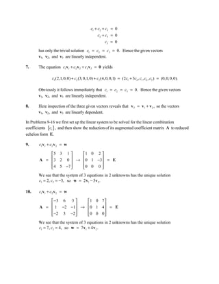
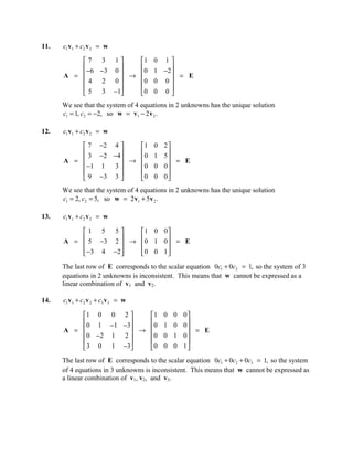
4. 15. c1v1 + c2 v 2 + c3 v 3 = w
 2 3 1 4 1 0 0 3 
 −1 0 2 5  → 0 1 0 −2  = E
A =    
 4 1 −1 6 
  0 0 1 4 
 
We see that the system of 3 equations in 3 unknowns has the unique solution
c1 = 3, c2 = −2, c3 = 4, so w = 3v1 − 2 v 2 + 4 v 3 .
16. c1v1 + c2 v 2 + c3 v 3 = w
2 4 1 7 1 0 0 6
0 1 3 7  0 1 0 −2 
A =  →   = E
3 3 −1 9  0 0 1 3
   
1 2 3 11 0 0 0 0
We see that the system of 4 equations in 3 unknowns has the unique solution
c1 = 6, c2 = −2, c3 = 3, so w = 6 v1 − 2 v 2 + 3v 3 .
In Problems 17-22, A = [ v1 v2 v 3 ] is the coefficient matrix of the homogeneous linear
system corresponding to the vector equation c1v1 + c2 v 2 + c3 v 3 = 0. Inspection of the indicated
reduced echelon form E of A then reveals whether or not a nontrivial solution exists.
1 2 3  1 0 0 
17. 0 −3 5  → 0 1 0  = E
A =    
1 4 2 
  0 0 1 
 
We see that the system of 3 equations in 3 unknowns has the unique solution
c1 = c2 = c3 = 0, so the vectors v1 , v 2 , v 3 are linearly independent.
 2 4 −2   1 0 −3 / 5 
18.  0 −5 1  → 0 1 −1/ 5  = E
A =    
 −3 −6 3 
  0 0
 0  
We see that the system of 3 equations in 3 unknowns has a 1-dimensional solution space.
If we choose c3 = 5 then c1 = 3 and c2 = 1. Therefore 3v1 + v 2 + 5 v3 = 0.
2 5 2  1 0 0
 0 4 −1  0
19. A =   → 0 1  = E
 3 −2 1  0 0 1
   
 0 1 −1 0 0 0

5. We see that the system of 4 equations in 3 unknowns has the unique solution
c1 = c2 = c3 = 0, so the vectors v1 , v 2 , v 3 are linearly independent.
1 2 3 1 0 0
1 1 
1 0 1 0
20. A =  →   = E
 −1 1 4 0 0 1
   
1 1 1 0 0 0
We see that the system of 4 equations in 3 unknowns has the unique solution
c1 = c2 = c3 = 0, so the vectors v1 , v 2 , v 3 are linearly independent.
3 1 1 1 0 1
 0 −1 
2 0 1 −2 
21. A =  →   = E
1 0 1 0 0 0
   
2 1 0 0 0 0
We see that the system of 4 equations in 3 unknowns has a 1-dimensional solution space.
If we choose c3 = −1 then c1 = 1 and c2 = −2. Therefore v1 − 2 v 2 − v 3 = 0.
3 3 5 1 0 7 / 9
9 0 
7 0 1 5 / 9
22. A =  →   = E
0 9 5 0 0 0 
   
5 −7 0 0 0 0 
We see that the system of 4 equations in 3 unknowns has a 1-dimensional solution space.
If we choose c3 = −9 then c1 = 7 and c2 = 5. Therefore 7 v1 + 5 v 2 − 9 v3 = 0.
23. Because v1 and v2 are linearly independent, the vector equation
c1u1 + c2u 2 = c1 ( v1 + v 2 ) + c2 ( v1 − v 2 ) = 0
yields the homogeneous linear system
c1 + c2 = 0
c1 − c2 = 0.
It follows readily that c1 = c2 = 0, and therefore that the vectors u1 and u2 are linearly
independent.
24. Because v1 and v2 are linearly independent, the vector equation
c1u1 + c2u 2 = c1 ( v1 + v 2 ) + c2 (2 v1 + 3v 2 ) = 0

6. yields the homogeneous linear system
c1 + 2c2 = 0
c1 + 3c2 = 0.
Subtraction of the first equation from the second one gives c2 = 0, and then it follows
from the first equation that c2 = 0 also. Therefore the vectors u1 and u2 are linearly
independent.
25. Because the vectors v1 , v 2 , v 3 are linearly independent, the vector equation
c1u1 + c2u 2 + c3u 3 = c1 ( v1 ) + c2 ( v1 + 2 v 2 ) + c3 ( v1 + 2 v 2 + 3v 3 ) = 0
yields the homogeneous linear system
c1 + c2 + c3 = 0
2c2 + 2c3 = 0
3c3 = 0.
It follows by back-substitution that c1 = c2 = c3 = 0, and therefore that the vectors
u1 , u 2 , u3 are linearly independent.
26. Because the vectors v1 , v 2 , v 3 are linearly independent, the vector equation
c1u1 + c2u 2 + c3u 3 = c1 ( v 2 + v 3 ) + c2 ( v1 + v 3 ) + c3 ( v1 + v 2 ) = 0
yields the homogeneous linear system
c2 + c3 = 0
c1 + c3 = 0
c1 + c2 = 0.
The reduction
0 1 1  1 0 0 
1 0 1  →  0 1 0  = E
A =    
1 1 0 
  0 0 1 
 
then shows that c1 = c2 = c3 = 0, and therefore that the vectors u1 , u 2 , u3 are linearly
independent.

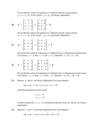
7. 27. If the elements of S are v1 , v 2 , , v k with v1 = 0, then we can take c1 = 1 and
c2 = = ck = 0. This choice gives coefficients c1 , c2 , , ck not all zero such that
c1v1 + c2 v 2 + + ck v k = 0. This means that the vectors v1 , v 2 , , v k are linearly
dependent.
28. Because the set S of vectors v1 , v 2 , , v k is linearly dependent, there exist scalars
c1 , c2 , , ck not all zero such that c1v1 + c2 v 2 + + ck v k = 0. If ck +1 = = cm = 0,
then c1 v1 + c2 v 2 + + cm v m = 0 with the coefficients c1 , c2 , , cm not all zero. This
means that the vectors v1 , v 2 , , v m comprising T are linearly dependent.
29. If some subset of S were linearly dependent, then Problem 28 would imply immediately
that S itself is linearly dependent (contrary to hypothesis).
30. Let W be the subspace of V spanned by the vectors v1 , v 2 , , v k . Because U is a
subspace containing each of these vectors, it contains every linear combination of
v1 , v 2 , , v k . But W consists solely of such linear combinations, so it follows that U
contains W.
31. If S is contained in span(T), then every vector in S is a linear combination of vectors in
T. Hence every vector in span(S) is a linear combination of linear combinations of
vectors in T. Therefore every vector in span(S) is a linear combination of vectors in T,
and therefore is itself in span(T). Thus span(S) is a subset of span(T).
32. If u is another vector in S then the k+1 vectors v1 , v 2 , , v k , u are linearly
dependent. Hence there exist scalars c1 , c2 , , ck , c not all zero such that
c1v1 + c2 v 2 + + ck v k + cu = 0. If c = 0 then we have a contradiction to the
hypothesis that the vectors v1 , v 2 , , v k are linearly independent. Therefore c ≠ 0,
so we can solve for u as a linear combination of the vectors v1 , v 2 , , v k .
33. The determinant of the k × k identity matrix is nonzero, so it follows immediately from
Theorem 3 in this section that the vectors v1 , v 2 , , v k are linearly independent.
34. If the vectors v1 , v 2 , , v n are linearly independent, then by Theorem 2 the matrix
A = [ v1 v 2 v n ] is nonsingular. If B is another nonsingular n × n matrix, then
the product AB is also nonsingular, and therefore (by Theorem 2) has linearly
independent column vectors.
35. Because the vectors v1 , v 2 , , v k are linearly independent, Theorem 3 implies that some
k × k submatrix A0 of A has nonzero determinant. Let A0 consist of the rows
i1 , i2 , , ik of the matrix A, and let C0 denote the k × k submatrix consisting of the

8. same rows of the product matrix C = AB. Then C0 = A0B, so C0 = A 0 B ≠ 0
because (by hypothesis) the k × k matrix B is also nonsingular. Therefore Theorem 3
implies that the column vectors of AB are linearly independent.