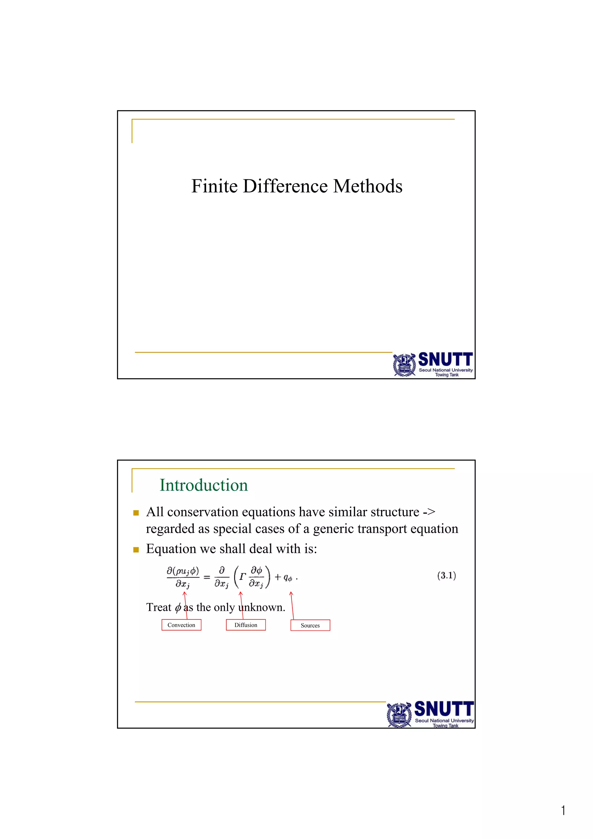
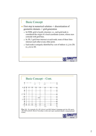
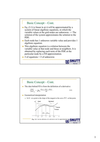
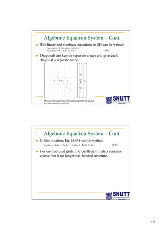
Finite difference methods discretize the domain into a grid and approximate derivatives as algebraic equations relating variable values at neighboring grid points. First and second derivatives can be approximated using forward, backward, or central differencing schemes of varying orders of accuracy. Boundary conditions require special treatment as higher-order approximations may require values outside the domain. Solving the resulting system of algebraic equations provides an approximate numerical solution to the partial differential equation over the discretized domain.

1. 1
Finite Difference Methods
Introduction
„ All conservation equations have similar structure ->
regarded as special cases of a generic transport equation
„ Equation we shall deal with is:
„ Equation we shall deal with is:
Treat φ as the only unknown.
Convection Diffusion Sources

2. 2
Basic Concept
„ First step in numerical solution -> discretization of
geometric domain -> grid generation
‰ In FDM grid is locally structure i e each grid node is
‰ In FDM, grid is locally structure, i.e., each grid node is
considered the origin of a local coordinate system, whose axes
coincide with grid lines.
‰ In 3D, 3 grid lines intersect at each node; none of these lines
intersect each other at any other point.
‰ Each node is uniquely identified by a set of indices: (i, j) in 2D;
(i j k) in 3D
(i, j, k) in 3D.
Basic Concept – Cont.

3. 3
Basic Concept – Cont.
„ Eq. (3.1) is linear in φ, it will be approximated by a
system of linear algebraic equations, in which the
variable values at the grid nodes are unknowns. -> The
solution of the system approximates the solution to the
PDE.
„ Each node has 1 unknown variable value and provides 1
algebraic equation.
„ This algebraic equation is a relation between the
variable value at that node and those at neighbors It is
variable value at that node and those at neighbors. It is
obtained by replacing each term of the PDE at the
particular node by a FD approximation.
„ # of equations = # of unknowns
Basic Concept – Cont.
„ The idea behind FD is from the definition of a derivative
„ Geometrical interpretation
‰ at a point is the slope of the tangent to the curve at that point.

4. 4
Basic Concept – Cont.
„ Some approximations are better than others.
„ Approximation quality improves when the additional
points are close to x In other words as the grid is
points are close to xi. In other words, as the grid is
refined, the approximation improves.
Approximation of the First Derivative
‰ For discretization of convective term
„ Taylor series expansion
‰ Any continuous differentiable function can be expressed as
‰ Any continuous differentiable function can be expressed as
a Taylor series, in the vicinity of xi,
‰ By replacing x by xi+1 or xi-1, we obtain expressions for the
variable values at these points in terms of the variable and its
derivatives at xi.

5. 5
First Derivative – Cont.
‰ Using these expressions, we can obtain approximate
expressions for 1st and higher derivatives at point xi in terms of
the function values at neighboring points.
‰ For example, (HW)
First Derivative – Cont.
‰ If the distance between grid points is small, HOTs will be
small.
‰ FDS
‰ BDS
‰ CDS

6. 6
First Derivative – Cont.
‰ Truncation error
„ Terms deleted from RHS
„ Sum of products of a power of the spacing and a higher derivative at
i HOT f E (3 4)
point compare HOTs of Eq. (3.4)
„ For example,
Note: α’s are higher-order derivatives multiplied by constant factors
Note: α s are higher-order derivatives multiplied by constant factors.
„ The order of an approximation indicates how fast the error is reduced
when the grid is refined; it does not indicate the absolute magnitude of
the error.
First Derivative – Cont.
„ Polynomial fitting
‰ Fit the function, φ, to an interpolation curve and differentiate
the resulting curve.
g
‰ Fitting a parabola to the data at xi-1, xi, and xi+1, and computing
the first derivative at xi from the interpolant, (HW)
‰ Second order truncation error; identical to CDS with uniform
i
spacing.
‰ In general, approximation of the first derivative possesses a
truncation error of the same order as the degree of the
polynomial used to approximate the function.

7. 7
First Derivative – Cont.
3rd order
by a cubic
polynomial
at 4 points
‰ In FDS and BDS, the major contribution to the approximation
comes from one side -> Upwind schemes (UDS).
4th order by
a 4-degree
polynomial
at 5 points
‰ 1st order UDS are very inaccurate, because of false diffusion.
‰ CDS can be easily implemented, since it is not necessary to
check the flow direction.
First Derivative – Cont.
„ Compact schemes
‰ Compact schemes can be derived through the use of
polynomial fitting.
p y g
‰ However, instead of using only the variable values at
computational nodes to derive the coefficients of the
polynomial, derivatives at some points are also used.
‰ 4th order Pade scheme
„ Use variable values at nodes, i, i+1, and i-1, and first derivatives at i+1
and i-1, to obtain approximation for the 1st derivative at i.
, pp
„ A polynomial of degree 4 in the vicinity of i:

8. 8
First Derivative – Cont.
„ Since we are interested in the first derivative at i, we only need to
compute a1.
„ Differentiating Eq. (3.15),
so that
„ By writing Eq. (3.15) for and Eq. (3.16)
for we obtain
First Derivative – Cont.
„ A family of compact centered approximations of up to 6 order
„ Obviously, for the same order of approximation, Pade schemes use
fewer computational nodes and thus have more compact computational
molecules than CDS.

9. 9
First Derivative – Cont.
„ Non-uniform grids
‰ Since the truncation error depends not only on the grid spacing
but also on the derivatives of the variable, we cannot achieve a
,
uniform distribution of discretization error on a uniform grid.
Æ We need to use a non-uniform grid.
‰ Use a smaller Δx in regions where derivatives of the function
are large and a larger Δx in regions where the function is
smooth. Æ Spread the error nearly uniformly over the domain.
‰ Even though different approximations are formally of the
‰ Even though different approximations are formally of the
same order for non-uniform spacing, they do not have the
same truncation error.
First Derivative – Cont.
‰ Leading truncation errors in CDS and FDS/BDS with grid
expansion ratio of re
‰ Grid refinement
„ Halving the spacing between 2 coarse grid points -> Grid becomes
uniform everywhere except near the coarsest grid points
„ Inserting new points so that the fine grid also has a constant ratio of
g p g
spacings

10. 10
First Derivative – Cont.
„ In the second case, the expansion factor of the fine grid is smaller than
on the coarse grid
„ At a common node the ratio of the leading truncation error
„ At a common node, the ratio of the leading truncation error
Then
„ rr is 4 when the grid is uniform,
„ rr > 4 when expanding or contracting
rr 4 when expanding or contracting
„ Generation of effective grids remains one of the most difficult problems
in CFD
Approximation of the Second Derivative
‰ For discretization of diffusion term
‰ Geometrically, slope of the line tangent to the curve
representing the first derivative
‰ All such approximations involve data from at least 3 points.
‰ FDS for outer derivative and BDS for inner derivative (HW)

11. 11
Second Derivative – Cont.
‰ A better choice is to evaluate at halfway points.
‰ The resulting expression (HW)
‰ For equidistant spacing,
Second Derivative – Cont.
‰ Yet another approach is using Taylor series expansion (HW)
‰ Increase the accuracy of approximations to the first derivatives,
using the second derivatives. Æ Keeping 2 RHS terms in Eq.
(3.4)
‰ Higher order approximations always involve more nodes,
yielding more complex equations to solve and more
complicated treatment of BCs, so a trade-off has to be made.

12. 12
Approximation of Mixed Derivatives
‰ Mixed derivatives occur only when the transport equations are
expressed in non-orthogonal coordinate systems.
‰ It may be treated by combining 1D approximations as for the
second derivative.
‰ The mixed second derivative at (xi, yi) can be estimated using
CDS by first evaluating the first derivative w.r.t. y at (xi+1, yj)
and (xi 1 yj)
and (xi-1, yj).
Implementation of Boundary Conditions
„ Continuous problem requires information about the solution at
the domain boundaries.
‰ Dirichlet: Variable value at the boundary
‰ Neumann: Variable’s gradient in a particular direction
‰ Combination of the above
„ Problem when higher order approximations of the derivatives are
used; since they require data at more than 3 points,
approximations at interior nodes may demand data at points
beyond the boundary.
„ It may then be necessary to use different approximations for the
derivatives at points close to boundary; usually these are of lower
order than the approximations used deeper in the interior and
may be one-sided differences.

13. 13
Boundary Conditions – Cont.
„ Examples
‰ Cubic polynomial fitting & 1st derivative at i=2
‰ 4th-order polynomial & 1st derivative at i=2
‰ Same polynomial & 2nd derivative
p y
Boundary Conditions – Cont.
„ If the gradient is prescribed at the boundary, a suitable
FD approximation for it (one-sided approximation) can
be used to compute the boundary value of the variable.
be used to compute the boundary value of the variable.
‰ Zero gradient in the normal direction, FDS leads to:
‰ Parabolic fit and 2 inner points, 2nd order approximation for 1st
derivative at the boundary

14. 14
Algebraic Equation System
„ FD approximation provides an algebraic equation at
each grid node.
„ It contains the variable value at that node as well as
„ It contains the variable value at that node as well as
values at neighboring nodes.
„ If the differential equation is non-linear, the
approximation will contain some non-linear terms. Æ
Linearization is required (Chap. 5)
„ For now consider only the linear case
„ For now, consider only the linear case.
Algebraic Equation System – Cont.
„ P and its neighbors form computational molecule.
„ A depend on geometrical quantities fluid properties
„ Al depend on geometrical quantities, fluid properties,
and variable values (for non-linear equations).
„ QP contain all the terms which do not contain unknown
variable values.

15. 15
Algebraic Equation System – Cont.
„ # equations must be equal to # of unknowns. In other
words, there has to be one equation for each grid node.
Æ Large set of linear algebraic equations, which must
Æ Large set of linear algebraic equations, which must
be solved numerically.
„ This system is sparse, meaning that each equation
contains only a few unknowns.
„ In matrix notation,
‰ A: square sparse coefficient matrix
‰ φ: vector containing variable values at grid nodes
‰ Q: vector containing RHS terms
Algebraic Equation System – Cont.
„ The structure of A depends on the ordering of variables in φ. For
structured grids, if the variables are labeled starting at a corner
and traversing line after line in a regular manner, the matrix has a
poly-diagonal structure.
„ For the case of 5-point molecule, all the non-zero coefficients lie
on the main diagonal, the two neighboring diagonals, and two
other diagonals removed by N positions from the main diagonal.
„ This system is sparse, meaning that each equation contains only a
few unknowns.
„ The variables are normally stored in computers in 1D arrays.
„

16. 16
Algebraic Equation System – Cont.
„ The linearized algebraic equations in 2D can be written
Di l k t i t d i h
„ Diagonals are kept in separate arrays and give each
diagonal a separate name.
Algebraic Equation System – Cont.
„ In this notation, Eq. (3.44) can be written
F t t d id th ffi i t t i i
„ For unstructured grids, the coefficient matrix remains
sparse, but it no longer has banded structure.

17. 17
Discretiztion Errors
„ Since the discretized equations represent approximations to the
differential equation, the exact solution of the latter, Φ, does not
satisfy the difference equation. Æ This imbalance is called
i
truncation error.
„ For a grid with a reference spacing h,
„ The exact solution of the discretized equations on grid h, φh,
satisfies
„ It differs from the exact solution of the PDE by the discretization
error, i.e.,
Discretiztion Errors – Cont.
„ From Eqs. (3.46) and (3.47),
‰ This equation states that the truncation error acts as a source of the
di i i hi h i d d diff d b h L
discretization error, which is convected and diffused by the operator Lh.
‰ Because the exact solution Φ is not known, the truncation error cannot be
calculated exactly.
„ For sufficiently fine grids, the truncation error (and discretization
error as well) is proportional to the leading term in the Taylor
series:
‰ H: HOT
‰ α: depends on the derivatives at the given point but is independent of h
‰ Note

18. 18
Discretiztion Errors – Cont.
„ The discretization error can be estimated from the difference
between solutions obtained on systematically refined grids.
„ Since the exact solution may be expressed as
„ p, which is the order of the scheme, may be estimated as (HW)
„ The discretization error on grid h can be approximated by (HW)
„ The order of convergence estimated using Eq. (3.52) is valid only
when the convergence is monotonic. Monotonic convergence is
expected only on sufficiently fine grids.
Examples
„ Read through and try yourself!