Sampling and low-rank tensor approximations

Sampling and Low-Rank Tensor Approximations
Hermann G. Matthies∗
Alexander Litvinenko∗
, Tarek A. El-Moshely+
∗
TU Braunschweig, Brunswick, Germany
+
MIT, Cambridge, MA, USA
wire@tu-bs.de
http://www.wire.tu-bs.de
$Id: 12_Sydney-MCQMC.tex,v 1.3 2012/02/12 16:52:28 hgm Exp $

2
Overview
1. Functionals of SPDE solutions
2. Computing the simulation
3. Parametric problems
4. Tensor products and other factorisations
5. Functional approximation
6. Emulation approximation
7. Examples and conclusion
TU Braunschweig Institute of Scientiﬁc Computing
CC
Scientifi omputing

3
Problem statement
We want to compute
Jk = E (Ψk(·, ue(·))) =
Ω
Ψk(ω, ue(ω)) P(dω),
where P is a probability measure on Ω, and
ue is the solution of a PDE depending on the parameter ω ∈ Ω.
A[ω](ue(ω)) = f(ω) a.s. in ω ∈ Ω,
ue(ω) is a U-valued random variable (RV).
To compute an approximation uM(ω) to ue(ω) via
simulation is expensive, even for one value of ω, let alone for
Jk ≈
N
n=1
Ψk(ωn, uM(ωn)) wn
Not all Ψk of interest are known from the outset.
CC
Scientifi omputing

4
Example: stochastic diﬀusion
Aquifer
0
0.5
1
1.5
2
0
0.5
1
1.5
2
Geometry
2D Model
Simple stationary model of groundwater ﬂow with stochastic data κ, f
− · (κ(x, ω) u(x, ω)) = f(x, ω) x ∈ D ⊂ Rd
& b.c.
Solution is in tensor space S ⊗ U =: W, e.g. W = L2(Ω, P) ⊗ ˚H1
(D)
leads after Galerkin discretisation with UM = span{vm}M
m=1 ⊂ U to
A[ω](uM(ω)) = f(ω) a.s. in ω ∈ Ω,
where uM(ω) =
M
m=1 um(ω)vm ∈ S ⊗ UM.
CC
Scientifi omputing

5
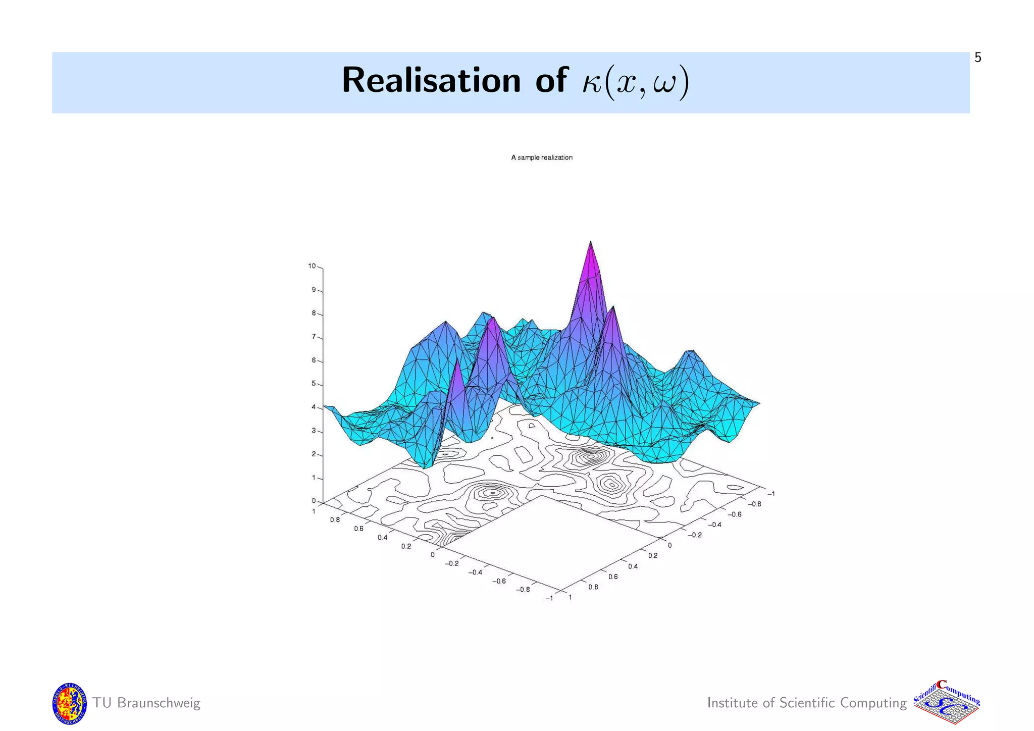
Realisation of κ(x, ω)
CC
Scientifi omputing

6
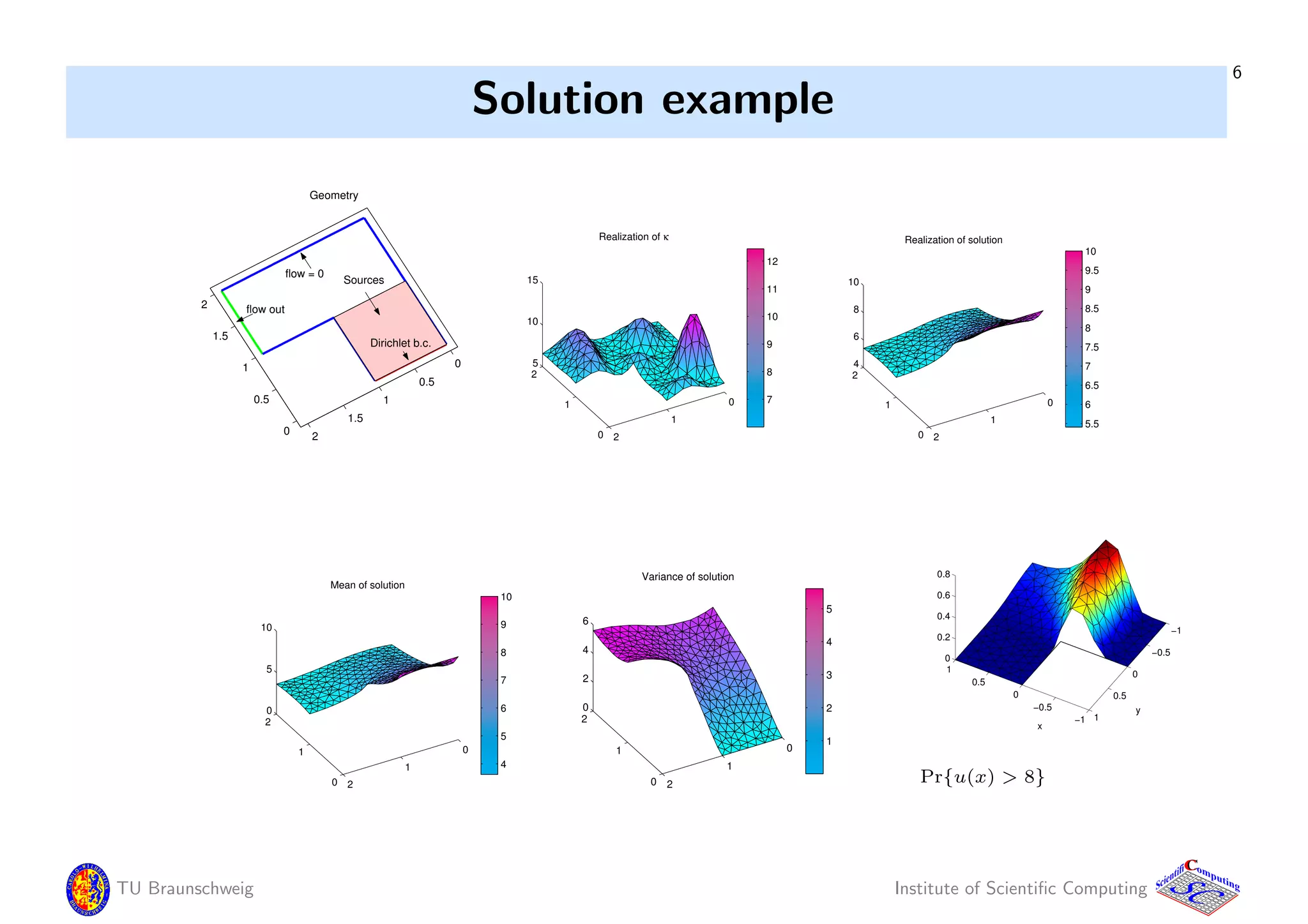
Solution example
0
0.5
1
1.5
2
0
0.5
1
1.5
2
Geometry
flow out
Dirichlet b.c.
flow = 0
Sources
7
8
9
10
11
12
0
1
2
0
1
2
5
10
15
Realization of κ
5.5
6
6.5
7
7.5
8
8.5
9
9.5
10
0
1
2
0
1
2
4
6
8
10
Realization of solution
4
5
6
7
8
9
10
0
1
2
0
1
2
0
5
10
Mean of solution
1
2
3
4
5
0
1
2
0
1
2
0
2
4
6
Variance of solution
−1
−0.5
0
0.5
1
−1
−0.5
0
0.5
1
0
0.2
0.4
0.6
0.8
y
x
Pr{u(x) > 8}
CC
Scientifi omputing

7
Computing the simulation
To simulate uM one needs samples of the random field (RF) κ,
which depends on infinitely many random variables (RVs).
This has to be reduced / transformed Ξ : Ω → [0, 1]s
to a finite number
s of RVs ξ = (ξ1, . . . , ξs), with µ = Ξ∗P the push-forward measure:
Jk =
Ω
Ψk(ω, ue(ω)) P(dω) ≈
[0,1]s
ˆΨk(ξ, uM(ξ)) µ(dξ).
This is a product measure for independent RVs (ξ1, . . . , ξs).
Approximate expensive simulation uM(ξ) by cheaper emulation.
Both tasks are related by viewing uM : ξ → uM(ξ), or κ1 : x → κ(x, ·)
(RF indexed by x), or κ2 : ω → κ(·, ω) (function valued RV),
maps from a set of parameters into a vector space.
CC
Scientifi omputing

8
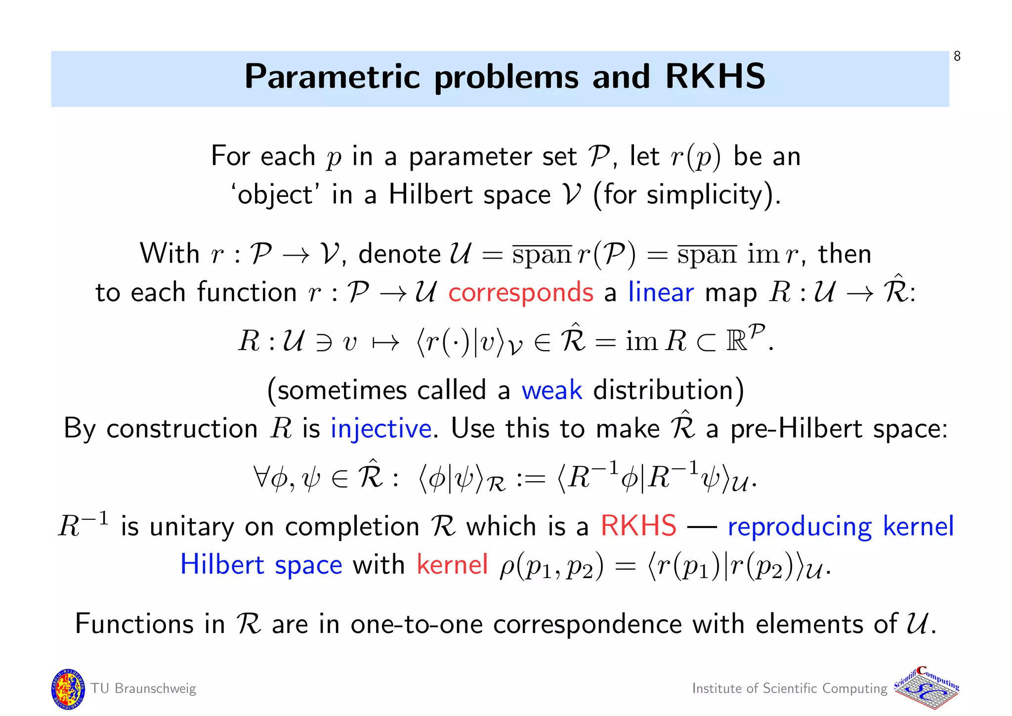
Parametric problems and RKHS
For each p in a parameter set P, let r(p) be an
‘object’ in a Hilbert space V (for simplicity).
With r : P → V, denote U = span r(P) = span im r, then
to each function r : P → U corresponds a linear map R : U → ˆR:
R : U v → r(·)|v V ∈ ˆR = im R ⊂ RP
.
(sometimes called a weak distribution)
By construction R is injective. Use this to make ˆR a pre-Hilbert space:
∀φ, ψ ∈ ˆR : φ|ψ R := R−1
φ|R−1
ψ U.
R−1
is unitary on completion R which is a RKHS — reproducing kernel
Hilbert space with kernel ρ(p1, p2) = r(p1)|r(p2) U.
Functions in R are in one-to-one correspondence with elements of U.
CC
Scientifi omputing

9
‘Covariance’
If Q ⊂ RP
is Hilbert with inner product ·|· Q; e.g. Q = L2(P, ν),
define in U a positive self-adjoint map—the covariance C = R∗
R
Cu|v U = Ru|Rv Q, ⇒ has spectrum σ(C) ⊆ R+,
with spectral projectors Eλ : C =
∞
0
λ dEλ
Similarly, define ˆC : Q → Q for φ, ψ ∈ Q such that ˆC = RR∗
by
ˆCφ|ψ Q = R∗
φ|R∗
ψ U ⇒ has same spectrum as C : σ( ˆC) = σ(C),
and unitarily equivalent projectors Êλ = WEλW∗
: ˆC =
∞
0
λ d Êλ.
Spectrum and projectors (σ(C), Eλ) are essence of r(p).
Specifically, for φ, ψ ∈ L2(P, ν) we have
R∗
φ|R∗
ψ U =
P×P
φ(p1)ρ(p1, p2)ψ(p2) ν(dp1) ν(dp2).
CC
Scientifi omputing

10
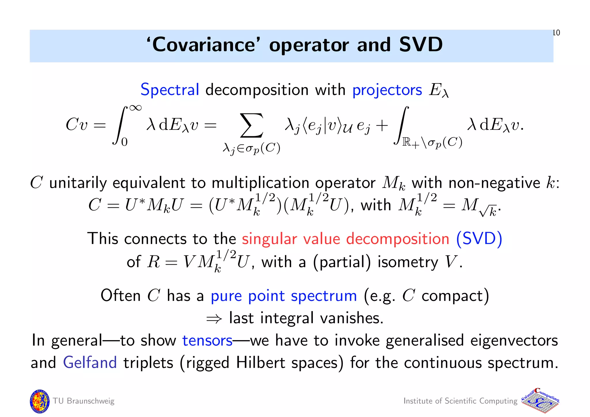
‘Covariance’ operator and SVD
Spectral decomposition with projectors Eλ
Cv =
∞
0
λ dEλv =
λj∈σp(C)
λj ej|v U ej +
R+σp(C)
λ dEλv.
C unitarily equivalent to multiplication operator Mk with non-negative k:
C = U∗
MkU = (U∗
M
1/2
k )(M
1/2
k U), with M
1/2
k = M√
k.
This connects to the singular value decomposition (SVD)
of R = V M
1/2
k U, with a (partial) isometry V .
Often C has a pure point spectrum (e.g. C compact)
⇒ last integral vanishes.
In general—to show tensors—we have to invoke generalised eigenvectors
and Gelfand triplets (rigged Hilbert spaces) for the continuous spectrum.
CC
Scientifi omputing

11
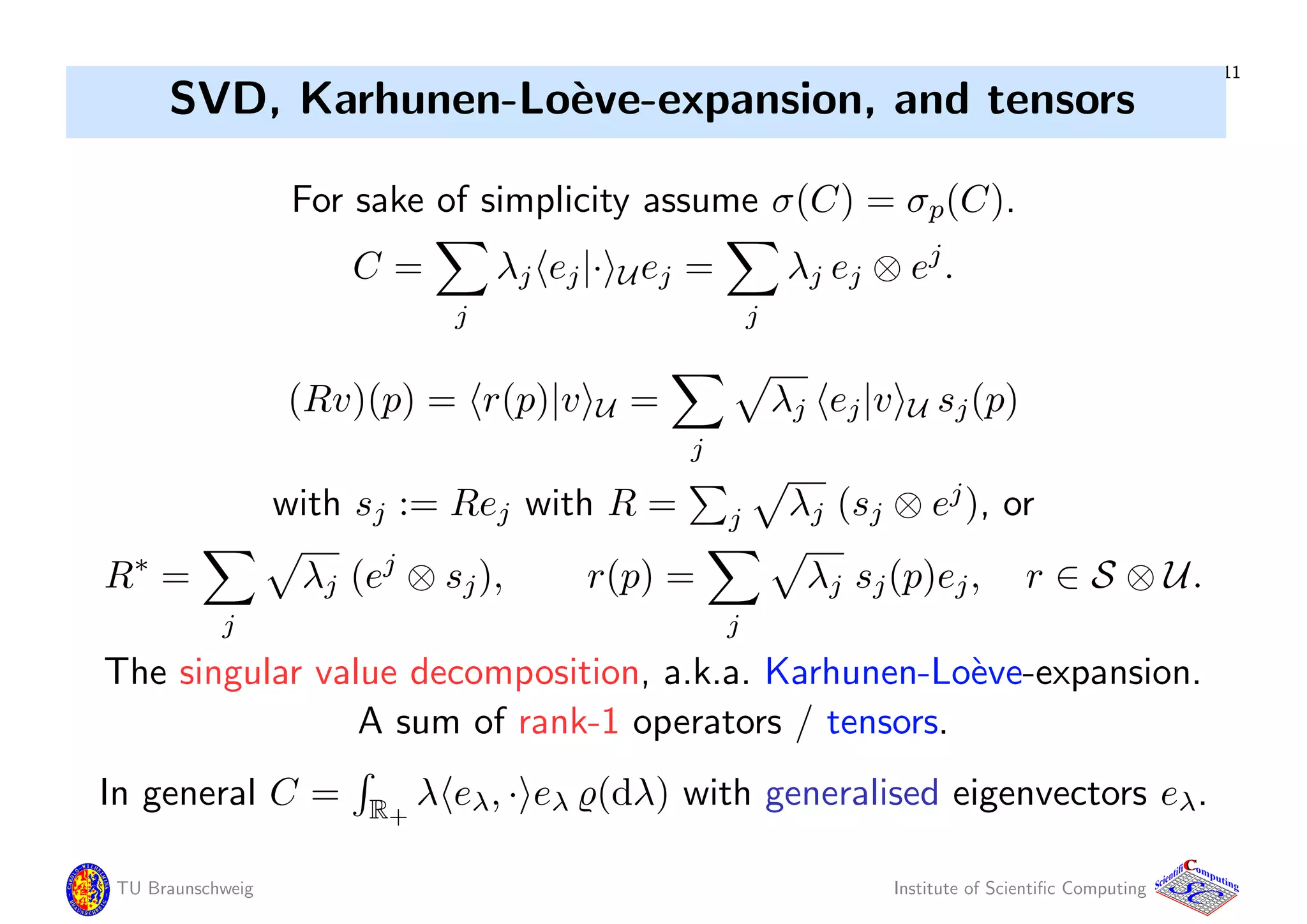
SVD, Karhunen-Lo`eve-expansion, and tensors
For sake of simplicity assume σ(C) = σp(C).
C =
j
λj ej|· Uej =
j
λj ej ⊗ ej
.
(Rv)(p) = r(p)|v U =
j
λj ej|v U sj(p)
with sj := Rej with R = j λj (sj ⊗ ej
), or
R∗
=
j
λj (ej
⊗ sj), r(p) =
j
λj sj(p)ej, r ∈ S ⊗ U.
The singular value decomposition, a.k.a. Karhunen-Lo`eve-expansion.
A sum of rank-1 operators / tensors.
In general C = R+
λ eλ, · eλ (dλ) with generalised eigenvectors eλ.
CC
Scientifi omputing

12
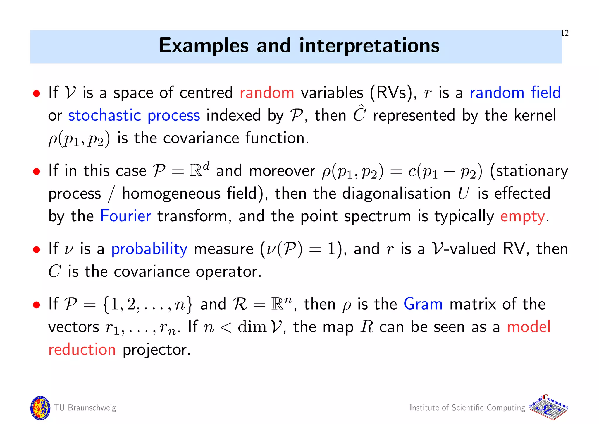
Examples and interpretations
• If V is a space of centred random variables (RVs), r is a random field
or stochastic process indexed by P, then ˆC represented by the kernel
ρ(p1, p2) is the covariance function.
• If in this case P = Rd
and moreover ρ(p1, p2) = c(p1 − p2) (stationary
process / homogeneous field), then the diagonalisation U is effected
by the Fourier transform, and the point spectrum is typically empty.
• If ν is a probability measure (ν(P) = 1), and r is a V-valued RV, then
C is the covariance operator.
• If P = {1, 2, . . . , n} and R = Rn
, then ρ is the Gram matrix of the
vectors r1, . . . , rn. If n < dim V, the map R can be seen as a model
reduction projector.
CC
Scientifi omputing

13
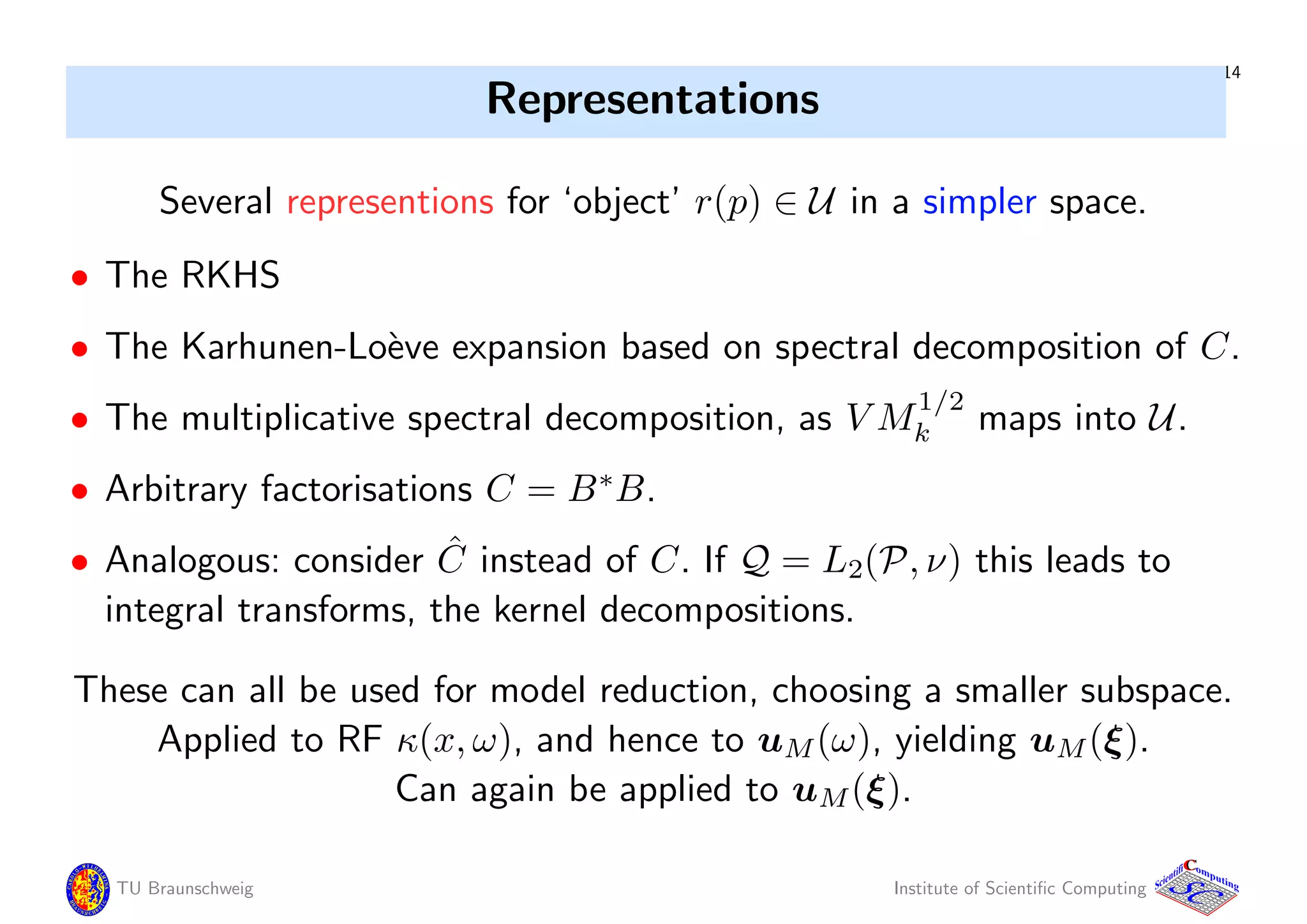
Factorisations / re-parametrisations
R∗
serves as representation for Karhunen-Lo`eve expansion.
This is a factorisation of C. Some other possible ones:
C = R∗
R = (V M
1/2
k )(V M
1/2
k )∗
= C1/2
C1/2
= B∗
B,
where C = B∗
B is an arbitrary one.
Each factorisation leads to a representation—all unitarily equivalent.
(When C is a matrix, a favourite is Cholesky: C = LL∗
).
Assume that C = B∗
B and B : U → H −→ r ∈ U ⊗ H.
Select a orthonormal basis {ek} in H.
Unitary Q : 2 a = (a1, a2, . . .) → k akek ∈ H.
Approximation possible by injection P∗
s : Rs
→ 2.
Let ˜r(a) := B∗
Qa := ˜R∗
a (linear in a), i.e. ˜R∗
: 2 → U. Then
˜R∗ ˜R = (B∗
Q)(Q∗
B) = B∗
B = C.
CC
Scientifi omputing

14
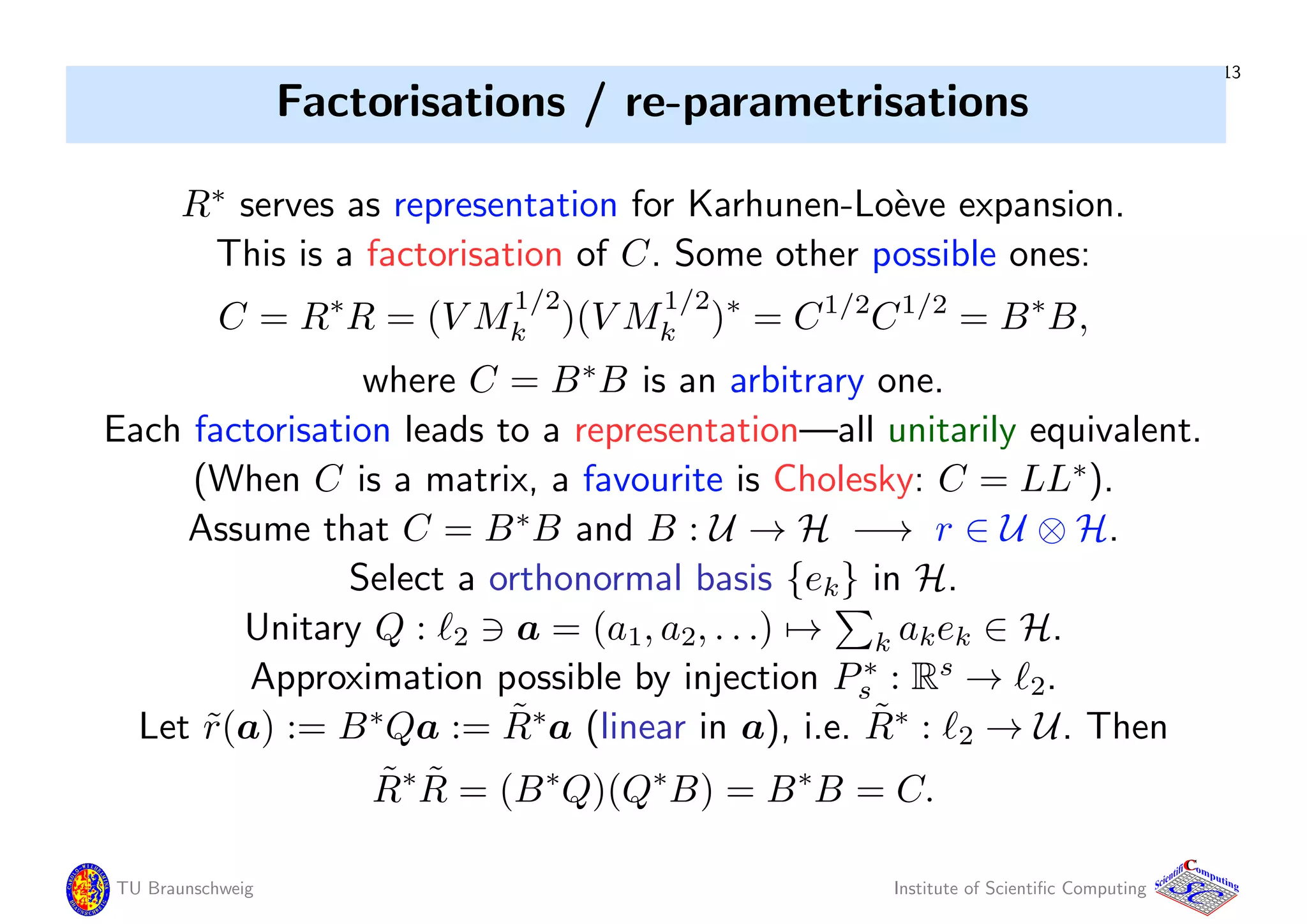
Representations
Several representions for ‘object’ r(p) ∈ U in a simpler space.
• The RKHS
• The Karhunen-Lo`eve expansion based on spectral decomposition of C.
• The multiplicative spectral decomposition, as V M
1/2
k maps into U.
• Arbitrary factorisations C = B∗
B.
• Analogous: consider ˆC instead of C. If Q = L2(P, ν) this leads to
integral transforms, the kernel decompositions.
These can all be used for model reduction, choosing a smaller subspace.
Applied to RF κ(x, ω), and hence to uM(ω), yielding uM(ξ).
Can again be applied to uM(ξ).
CC
Scientifi omputing

15
Functional approximation
Emulation — replace expensive simulation uM(ξ) by inexpensive
approximation / emulation uE(ξ) ≈ uM(ξ)
( alias response surfaces, proxy / surrogate models, etc.)
Choose subspace SB ⊂ S with basis {Xβ}B
β=1,
make ansatz for each um(ξ) ≈ β uβ
mXβ(ξ), giving
uE(ξ) =
m,β
uβ
mXβ(ξ)vm =
m,β
uβ
mXβ(ξ) ⊗ vm.
Set U = (uβ
m) — (M × B).
Sampling, we generate matrix / tensor
U = [uM(ξ1), . . . , uM(ξN)] = (um(ξn))n
m — (M × N).
CC
Scientifi omputing

16
Tensor product structure
Story does not end here as one may choose S = k Sk,
approximated by SB =
K
k=1 SBk
, with SBk
⊂ Sk.
Solution represented as a tensor of grade K + 1
in WB,N =
K
k=1 SBk
⊗ UN.
For higher grade tensor product structure, more reduction is possible,
— but that is a story for another talk, here we stay with K = 1.
With orthonormal Xβ one has
uβ
m =
[0,1]s
Xβ(ξ)um(ξ) µ(dξ) ≈
N
n=1
wnXβ(ξn)um(ξn).
Let W = diag (wn)—(N × N), X = (Xβ(ξn)) — (B × N), hence
U = U(W XT
). For B = N this is just a basis change.
CC
Scientifi omputing

17
Low-rank approximation
Focus on array of numbers U := [um(ξn)], view as matrix / tensor:
N
n=1
M
m=1
Um,nem
M ⊗ en
N, with unit vectors en
N ∈ RN
, em
M ∈ RM
.
The sum has M ∗ N terms, the number of entries in U.
Rank-R representation is approximation with R terms
U =
N
n=1
M
m=1
Um,nem
M(en
N)T
≈
R
=1
a bT
= ABT
,
with A = [a1, . . . , aR] — (M × R) and B = [b1, . . . , bR] — (N × R).
It contains only R ∗ (M + N) M ∗ N numbers.
We will use updated, truncated SVD. This gives for coeﬃcients
U = U(W XT
) ≈ ABT
(W XT
) = A(XW B)T
=: AB
T
CC
Scientifi omputing

18
Emulation instead of simulation
Let x(ξ) := [X1(ξ), . . . , XB(ξ)]T
. Emulator and low-rank emulator is
uE(ξ) = Ux(ξ), and uL(ξ) := AB
T
x(ξ).
Computing A, B: start with z samples Uz1 = [uM(ξ1), . . . , uM(ξz)].
Compute truncated, error controled SVD:
M×z
Uz1 ≈
M×R
W
R×R
Σ
z×R
V
T
;
then set A1 = W Σ1/2
, B1 = V Σ1/2
⇒ B1.
For each n = z + 1, . . . , 2z, emulate uL(ξn) and evaluate residuum
rn := r(ξn) := f(ξn) − A[ξn](uL(ξn)). If rn is small, accept
un
A = uL(ξn), otherwise solve for uM(ξn) and set un
A = uM(ξn).
Set Uz2 = [uz+1
A , . . . , u2z
A ], compute updated SVD of [Uz1, Uz2],
⇒ A2, B2. Repeat for each batch of z samples.
CC
Scientifi omputing

19
Emulator in integration
To evaluate
Jk =
Ω
Ψk(ω, ue(ω)) P(dω) ≈
[0,1]s
ˆΨk(ξ, uM(ξ)) µ(dξ),
we compute
Jk ≈
N
n=1
wn
ˆΨk(ξn, uL(ξn)).
If we are lucky, we need much fewer than N samples to ﬁnd the
low-rank representation A, B for uL.
This is cheap to compute from samples, and uses only little storage.
In the integral the integrand is cheap to evaluate, and the low-rank
representation can be re-used if a new (Jk, Ψk) has to be evaluated.
CC
Scientifi omputing

20
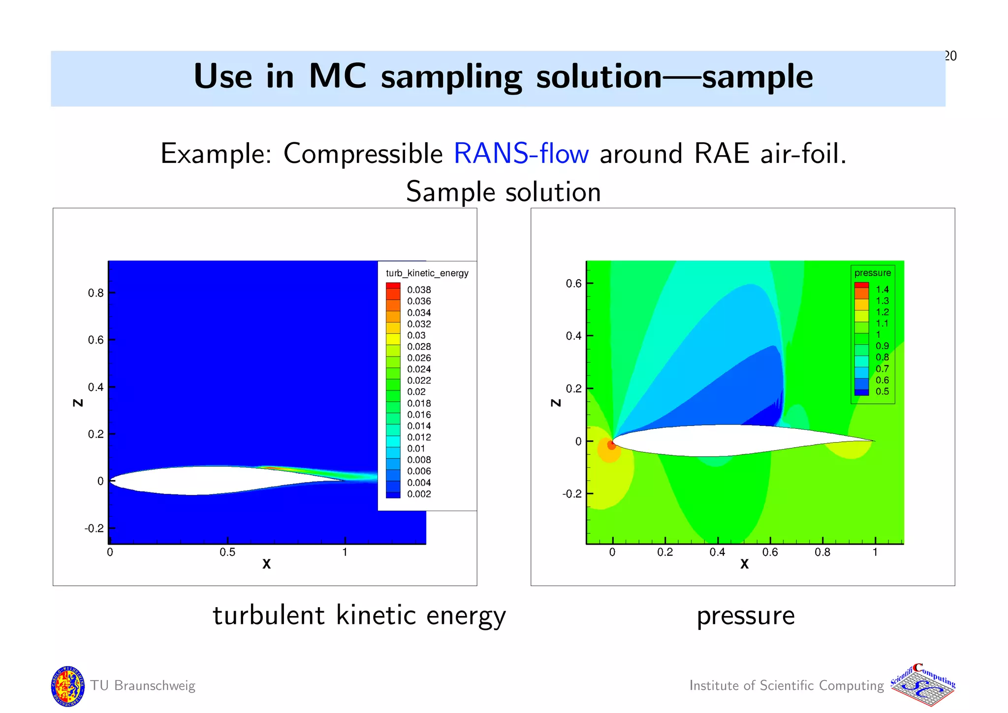
Use in MC sampling solution—sample
Example: Compressible RANS-ﬂow around RAE air-foil.
Sample solution
turbulent kinetic energy pressure
CC
Scientifi omputing

21
Use in MC sampling solution—storage
Inﬂow and air-foil shape uncertain.
Data compression achieved by updated SVD:
Made from 600 MC Simulations, SVD is updated every 10 samples.
M = 260, 000 N = 600
Updated SVD: Relative errors, memory requirements:
rank R pressure turb. kin. energy memory [MB]
10 1.9e-2 4.0e-3 21
20 1.4e-2 5.9e-3 42
50 5.3e-3 1.5e-4 104
Dense matrix ∈ R260000×600
costs 1250 MB storage.
CC
Scientifi omputing

22
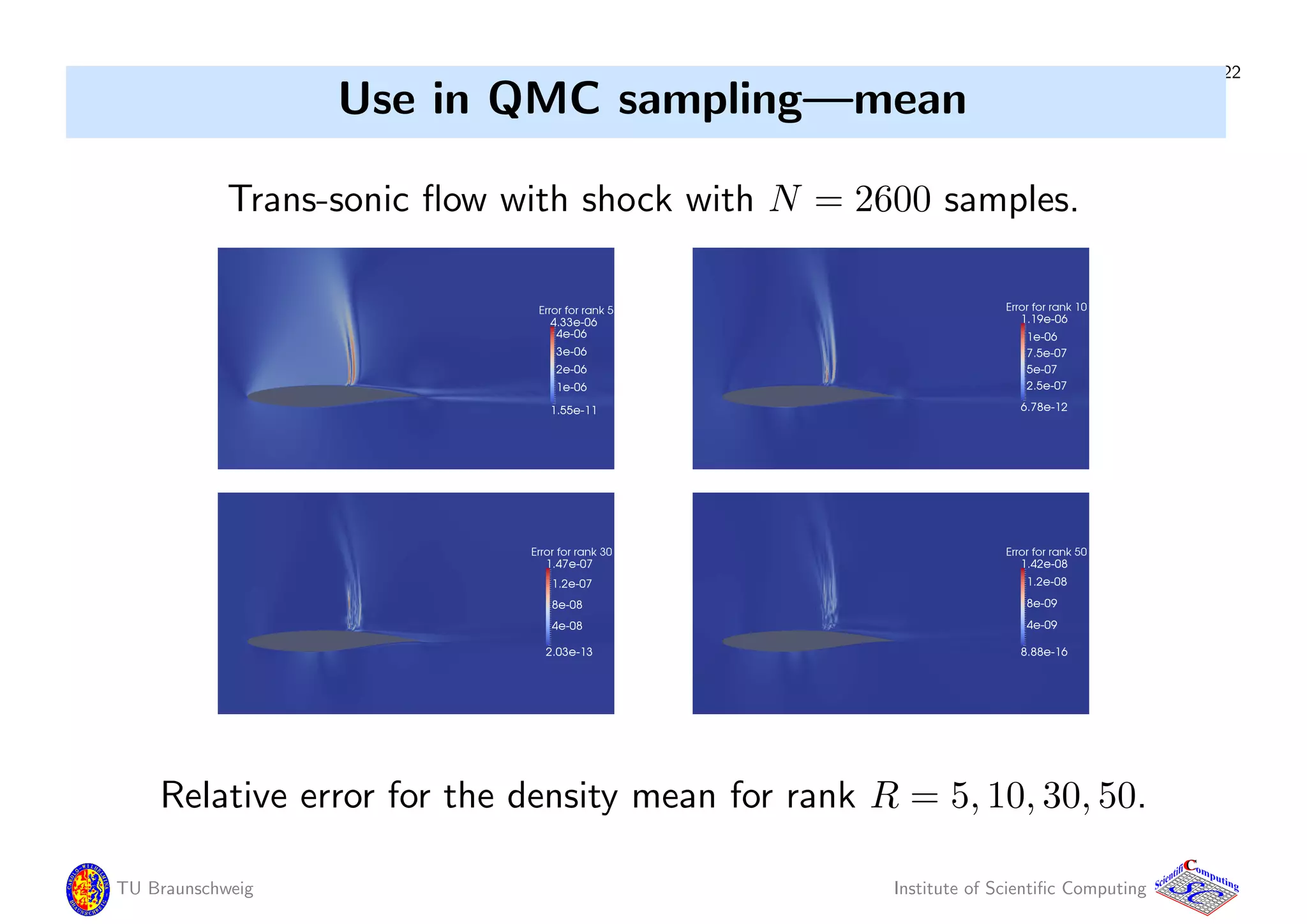
Use in QMC sampling—mean
Trans-sonic ﬂow with shock with N = 2600 samples.
Relative error for the density mean for rank R = 5, 10, 30, 50.
CC
Scientifi omputing

23
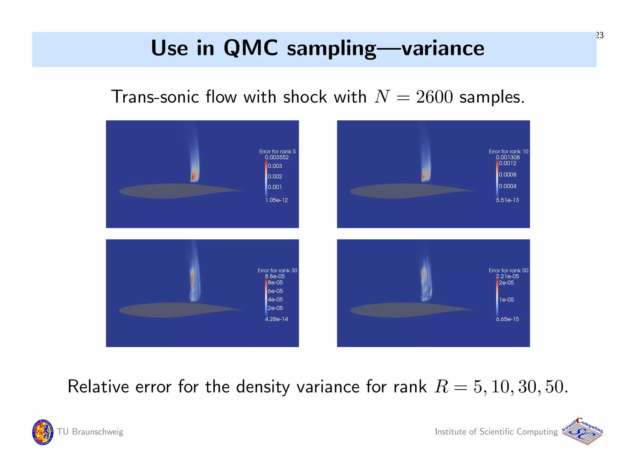
Use in QMC sampling—variance
Trans-sonic ﬂow with shock with N = 2600 samples.
Relative error for the density variance for rank R = 5, 10, 30, 50.
CC
Scientifi omputing

24
Conclusion
• Random ﬁeld discretisation and sampling can be seen as weak
distribution with associated covariance.
• Analysis of associated linear map reveals essential structure.
• Factorisations of covariance lead to SVD (Karhunen-Lo`eve
expansion) and tensor products.
• Functional approximation to construct emulator.
• Sparse and inexpensive emulation.
CC
Scientifi omputing

Sampling and low-rank tensor approximations

More Related Content

What's hot

Viewers also liked

Similar to Sampling and low-rank tensor approximations

More from Alexander Litvinenko

Recently uploaded

Sampling and low-rank tensor approximations