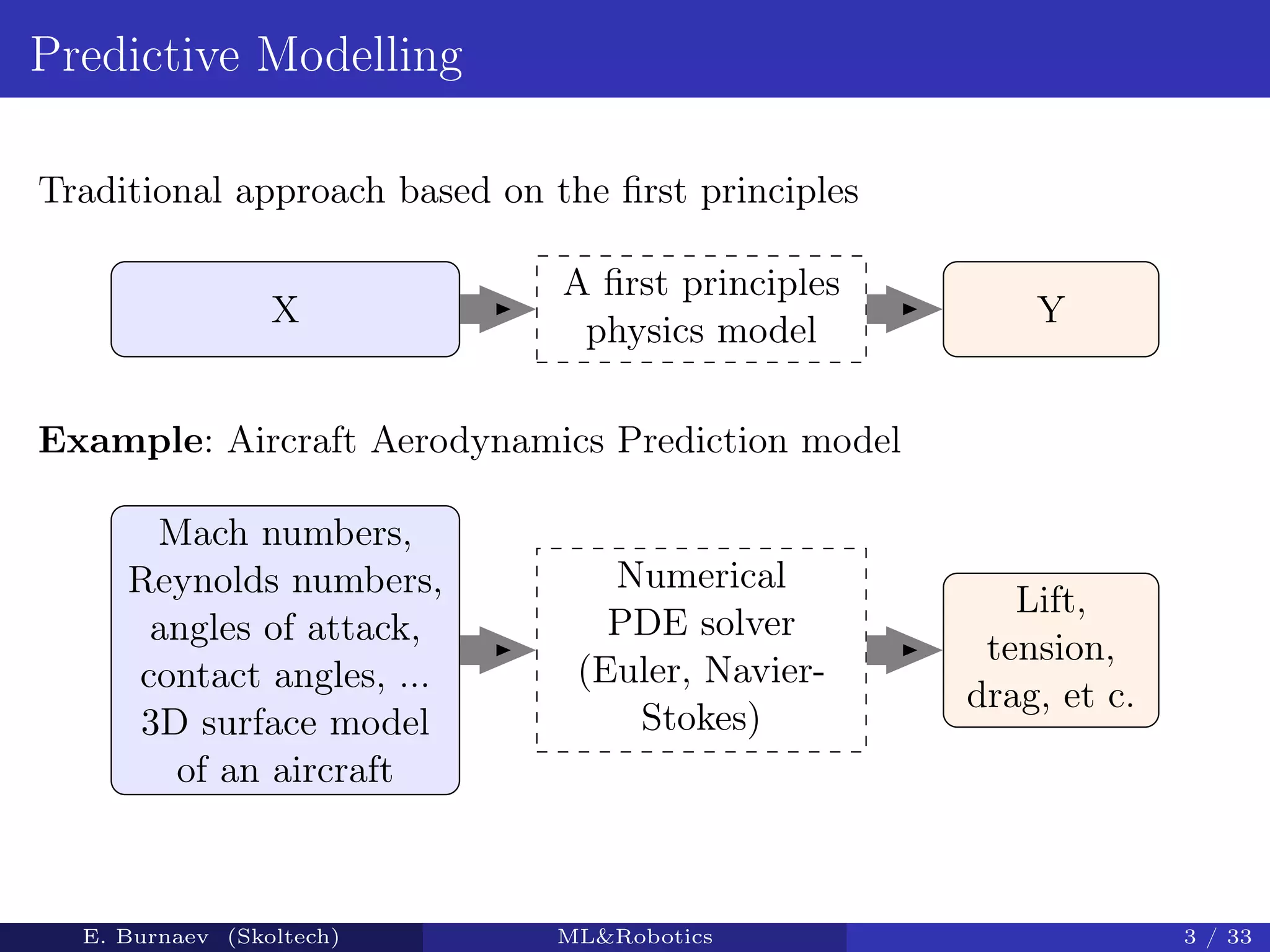
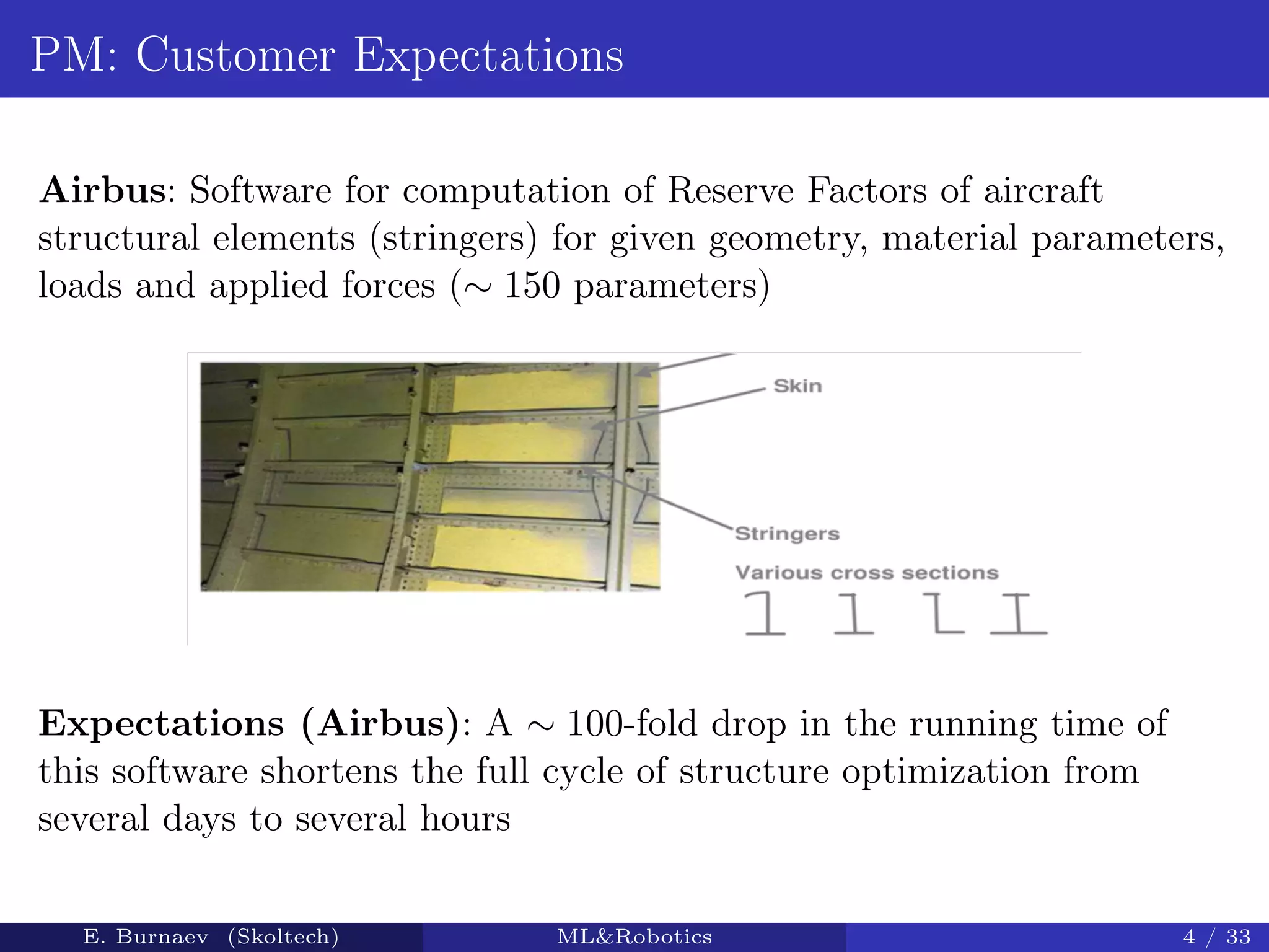
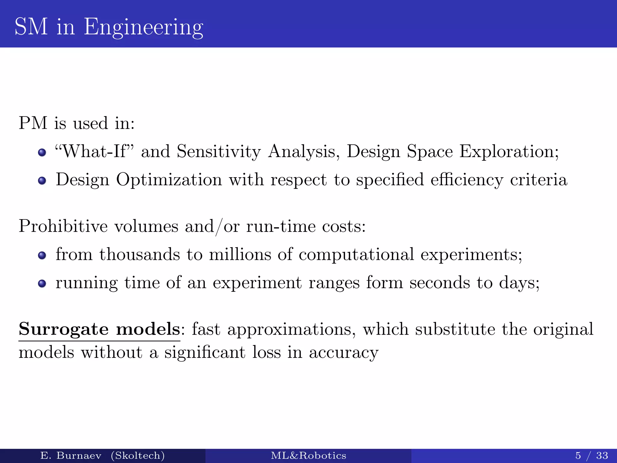
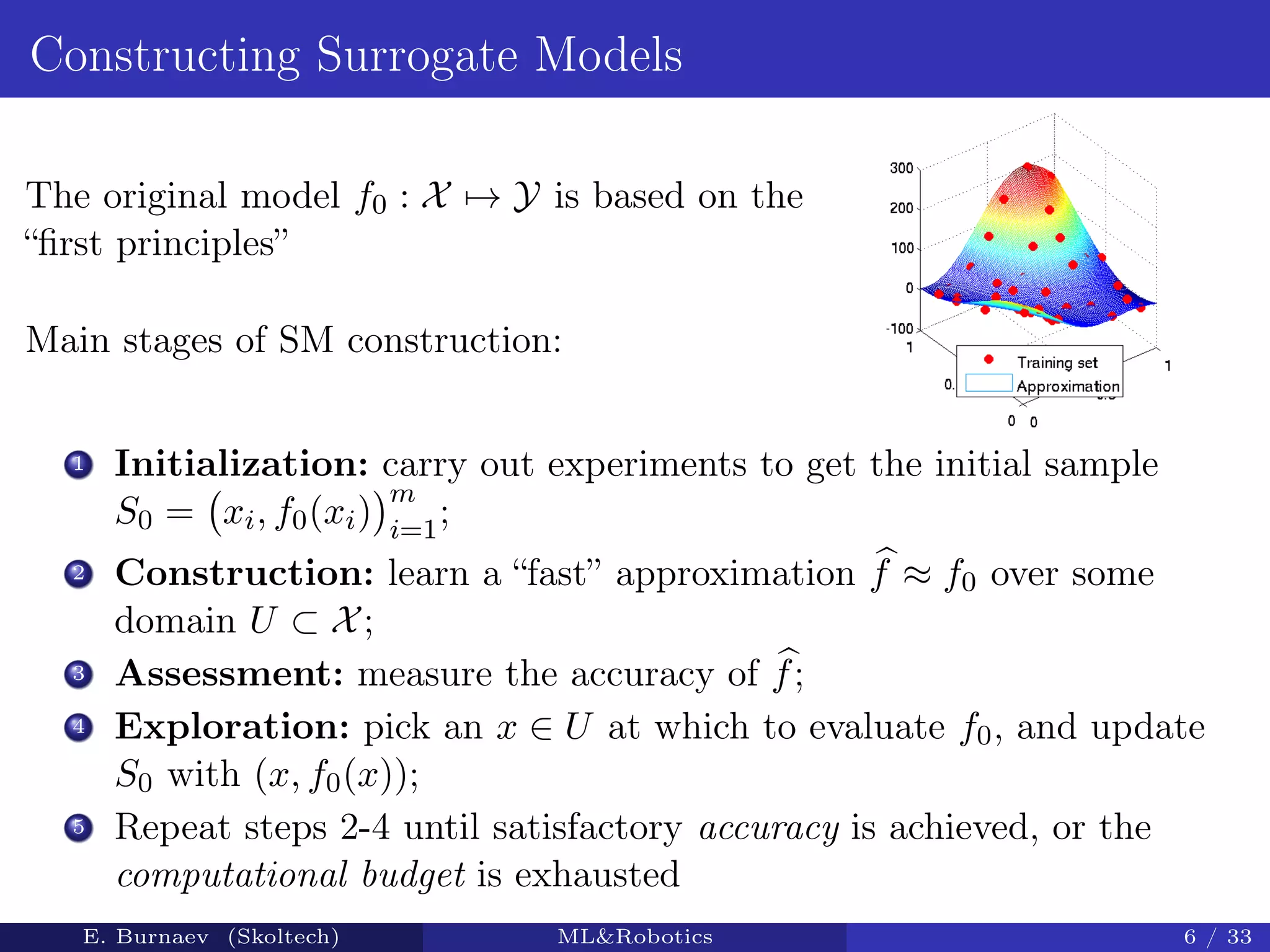
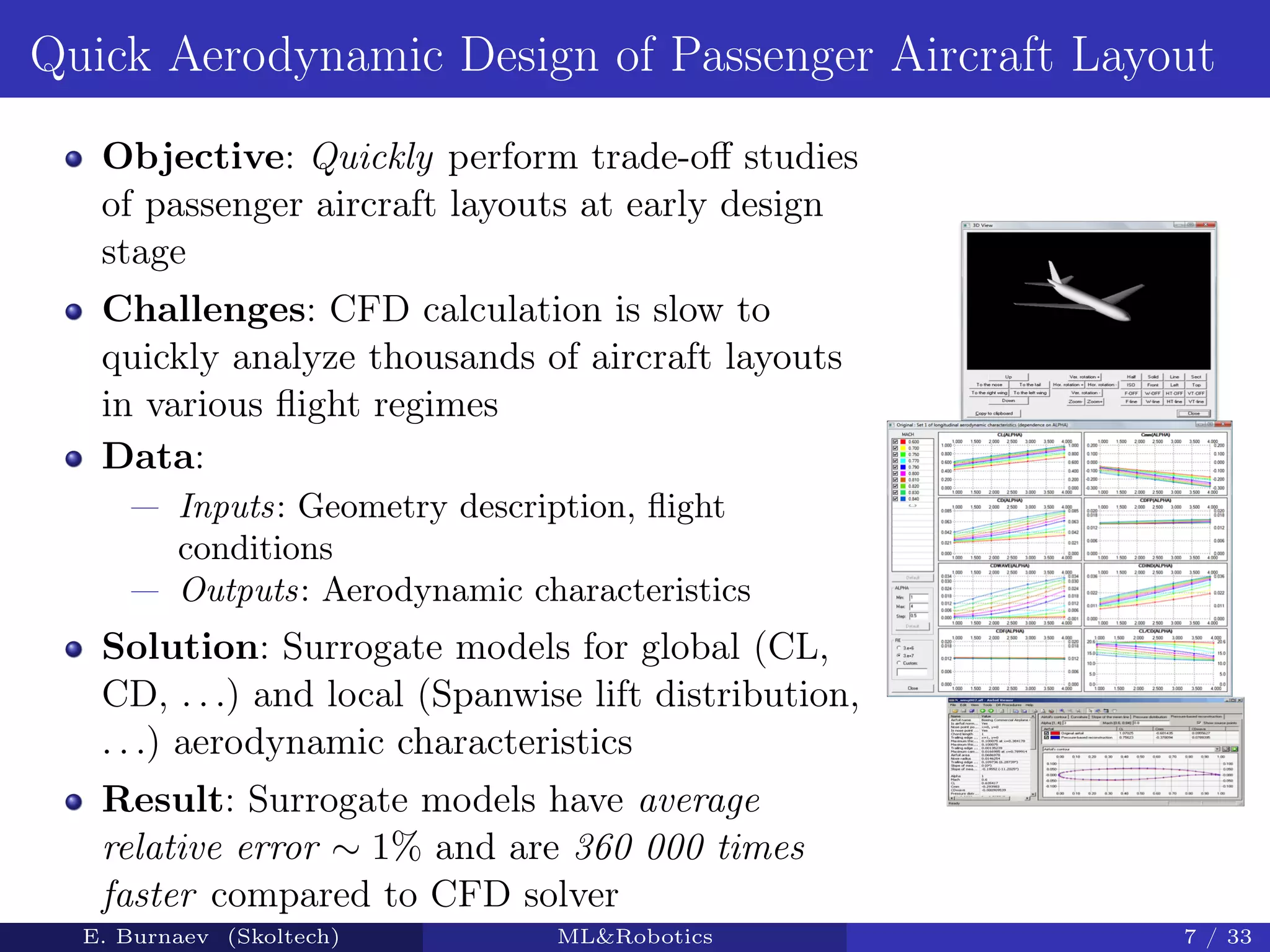
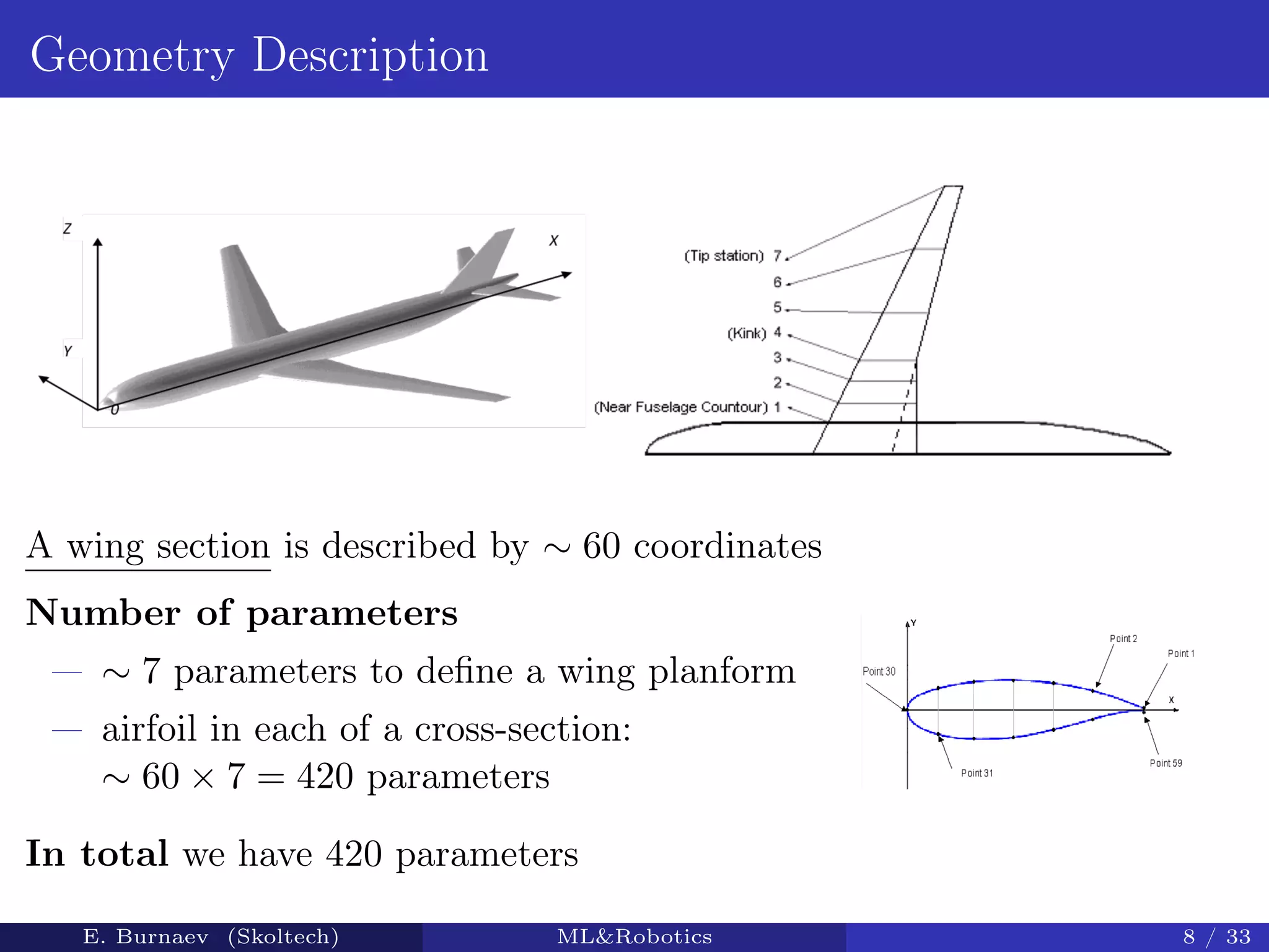
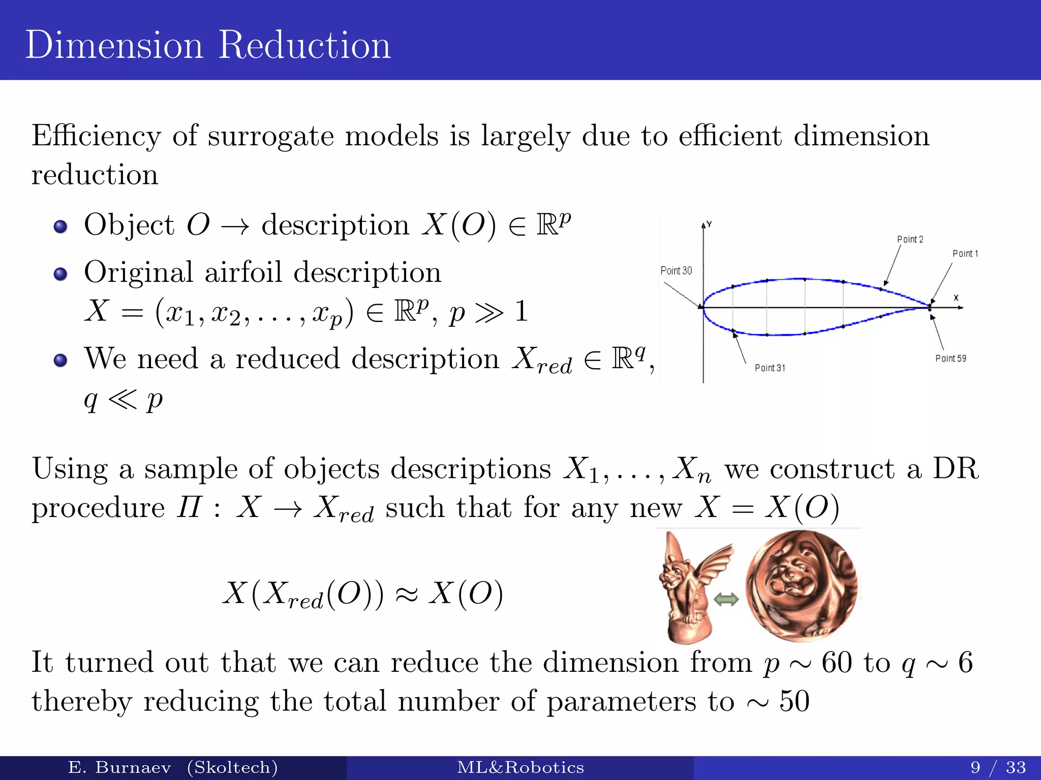
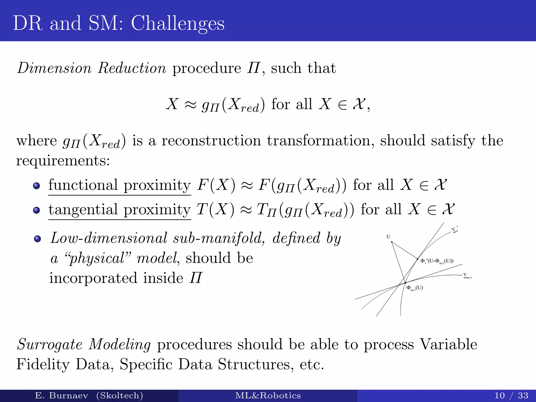
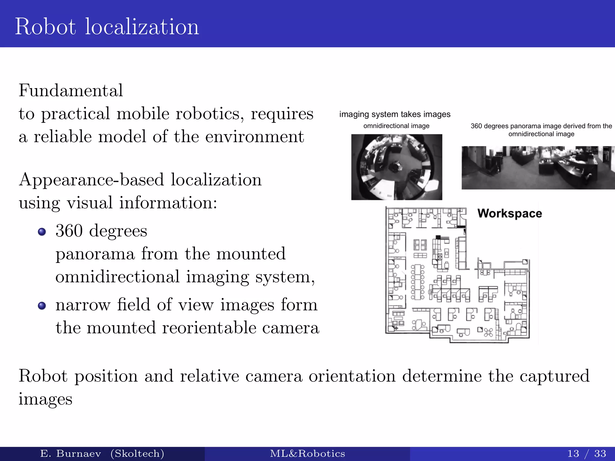
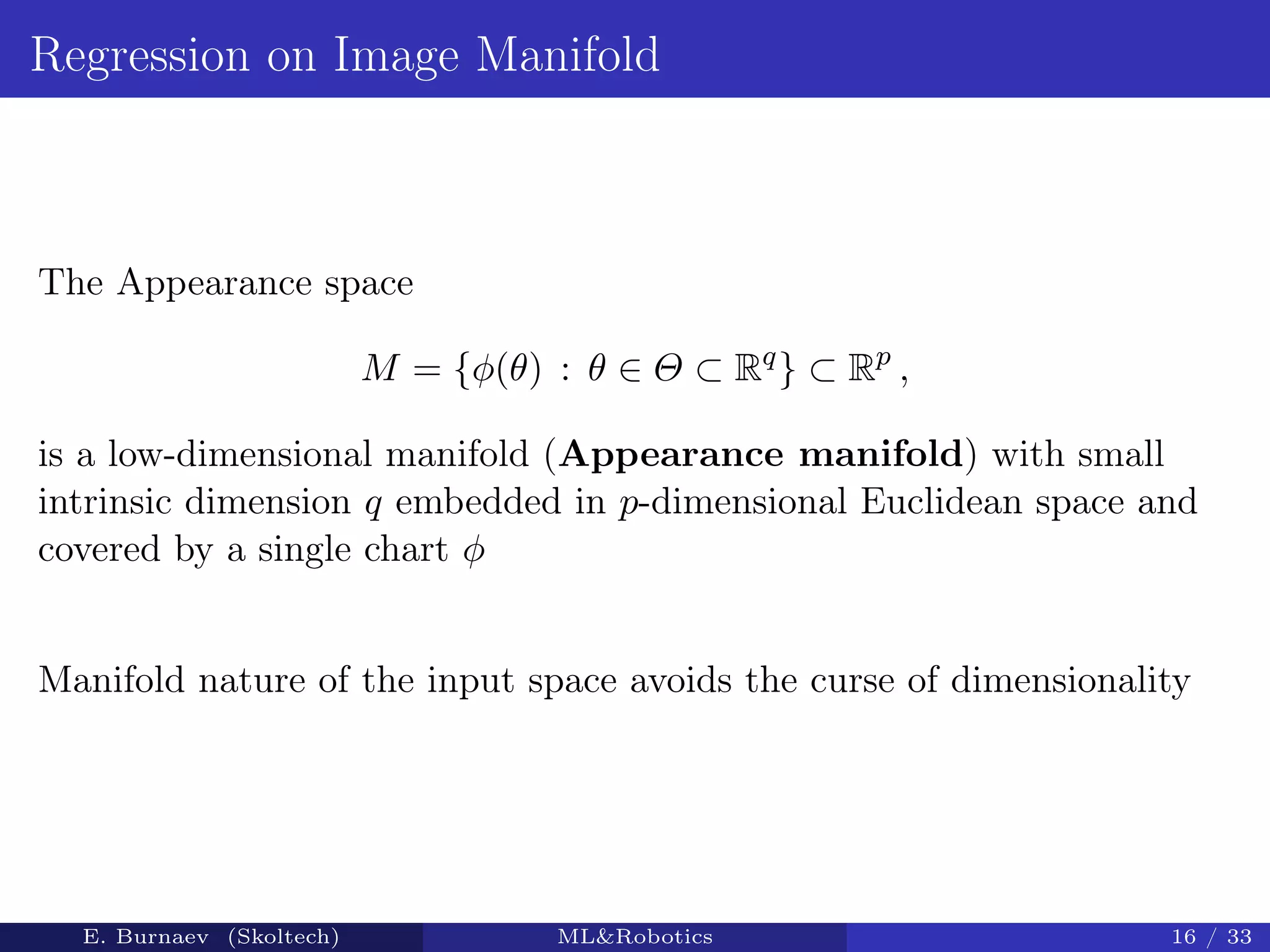
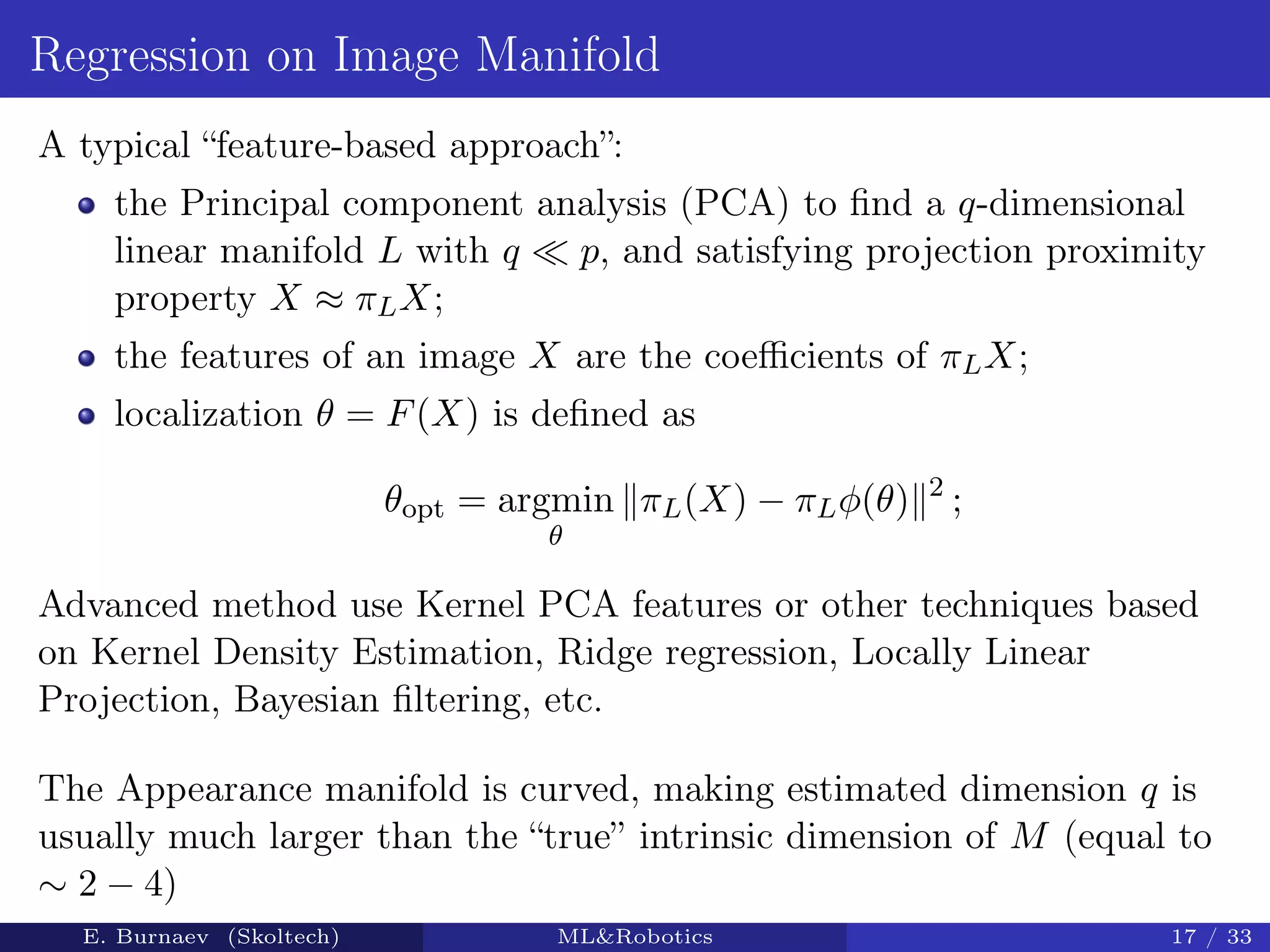
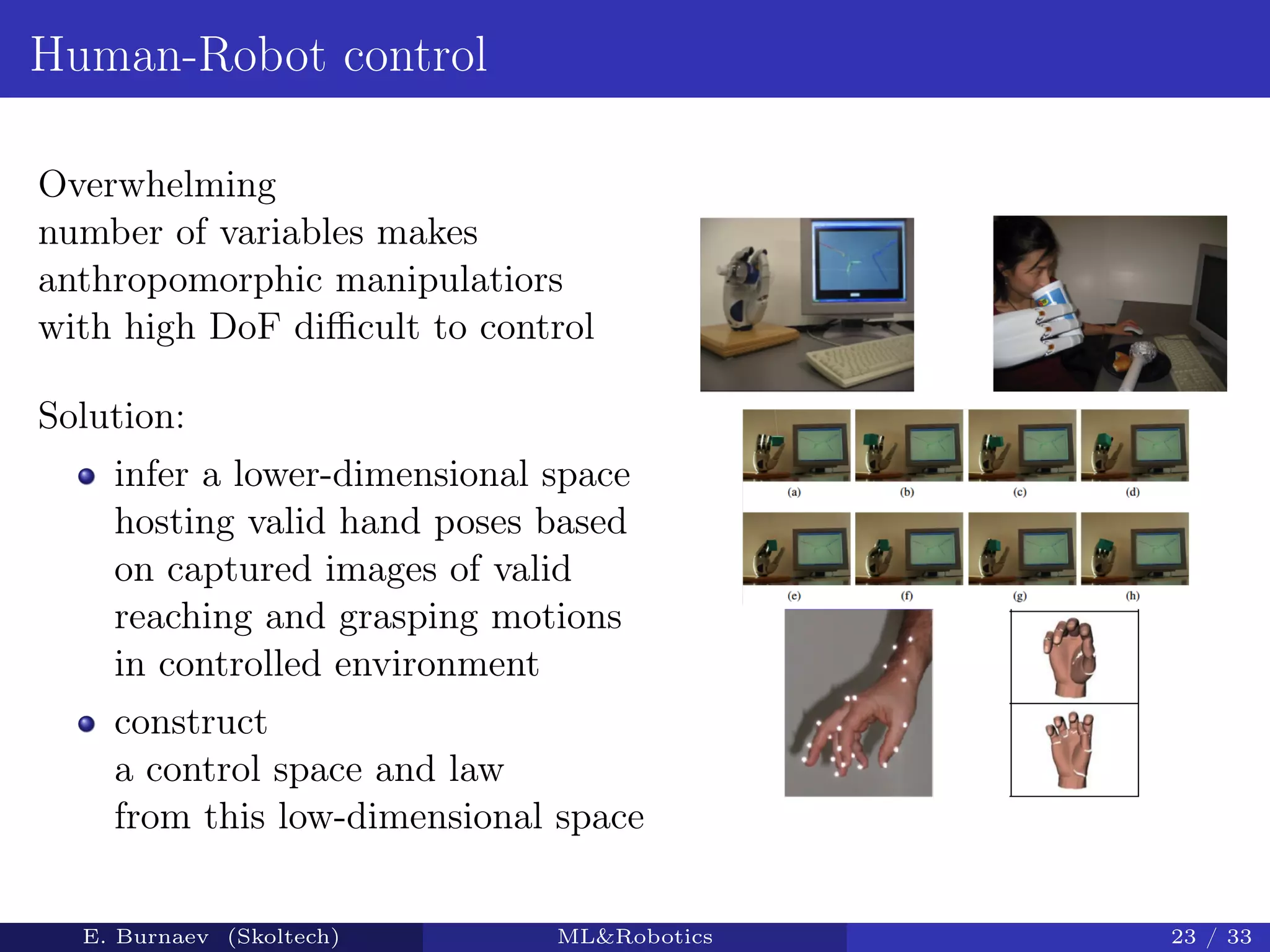
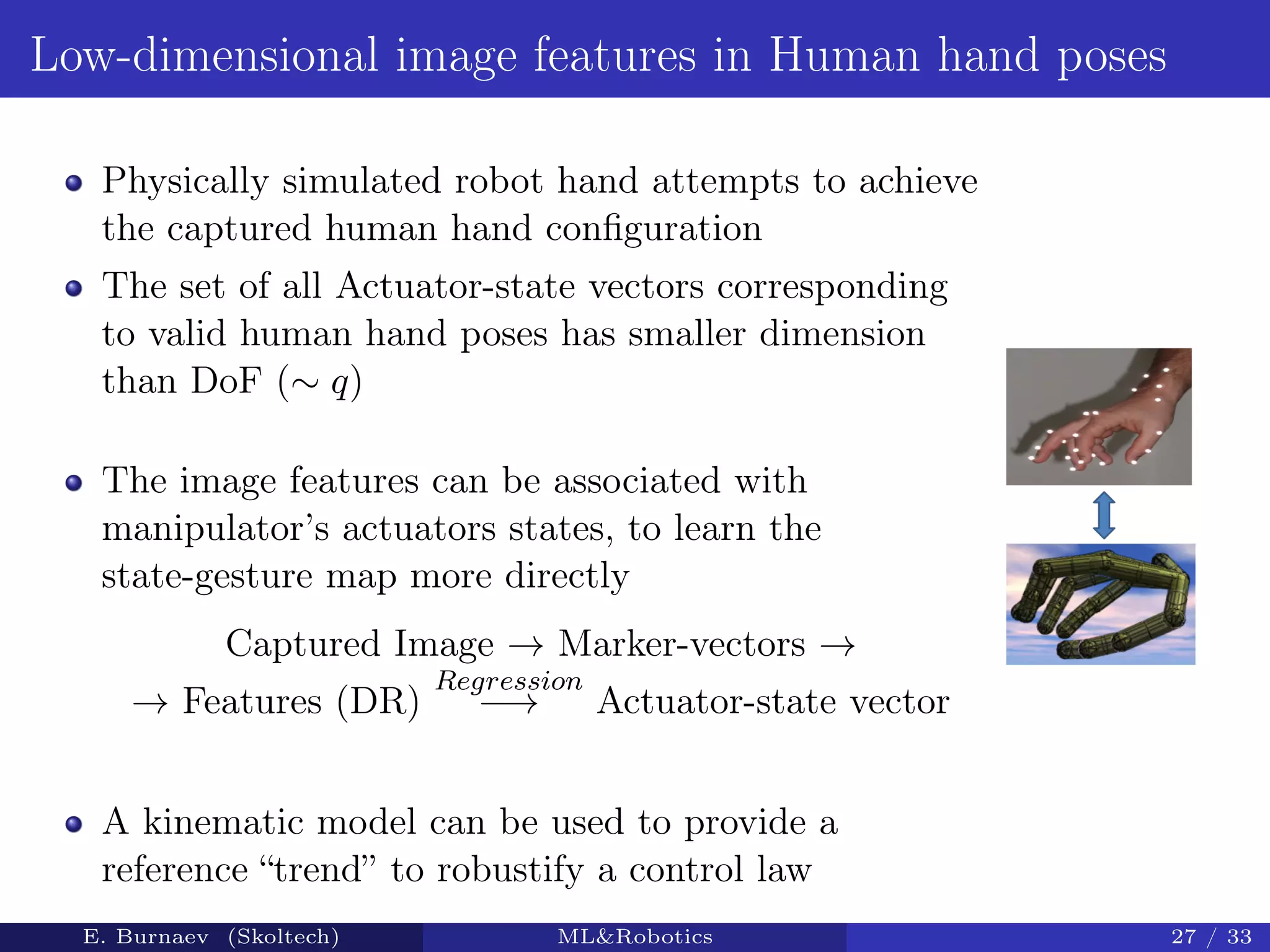
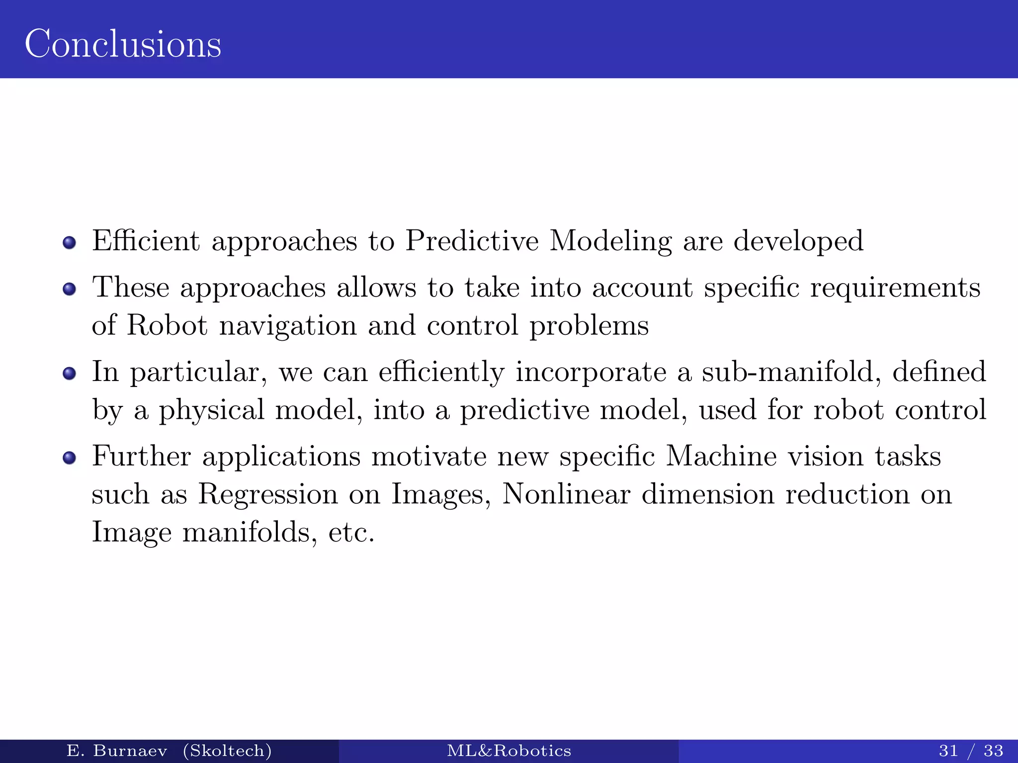
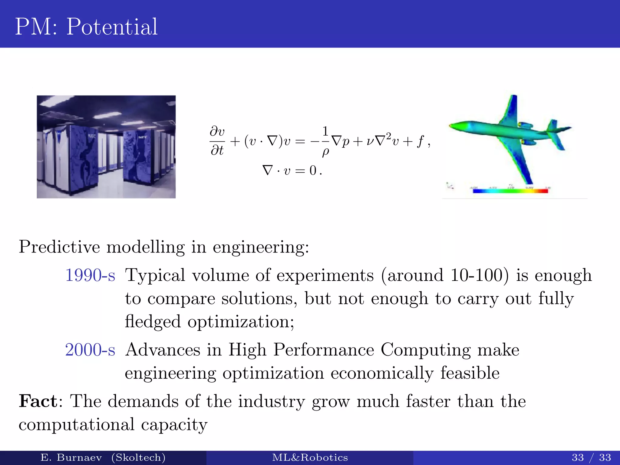
Применение машинного обучения для навигации и управления роботами
1. Machine Learning Applications for
Robot Navigation and Control
E. Burnaev
Skoltech
E. Burnaev (Skoltech) ML&Robotics 1 / 33
2. Outline
1 Predictive Modelling in Industrial Engineering
Predictive Modelling
Customer Expectations
Surrogate Models
Dimension Reduction
2 Robot navigation
3 ML problem statement
4 Robot control
5 Conclusions
E. Burnaev (Skoltech) ML&Robotics 2 / 33
3. Predictive Modelling
Traditional approach based on the first principles
A first principles
physics model
X Y
Example: Aircraft Aerodynamics Prediction model
Numerical
PDE solver
(Euler, Navier-
Stokes)
Mach numbers,
Reynolds numbers,
angles of attack,
contact angles, ...
3D surface model
of an aircraft
Lift,
tension,
drag, et c.
E. Burnaev (Skoltech) ML&Robotics 3 / 33
4. PM: Customer Expectations
Airbus: Software for computation of Reserve Factors of aircraft
structural elements (stringers) for given geometry, material parameters,
loads and applied forces (∼ 150 parameters)
Expectations (Airbus): A ∼ 100-fold drop in the running time of
this software shortens the full cycle of structure optimization from
several days to several hours
E. Burnaev (Skoltech) ML&Robotics 4 / 33
5. SM in Engineering
PM is used in:
“What-If” and Sensitivity Analysis, Design Space Exploration;
Design Optimization with respect to specified efficiency criteria
Prohibitive volumes and/or run-time costs:
from thousands to millions of computational experiments;
running time of an experiment ranges form seconds to days;
Surrogate models: fast approximations, which substitute the original
models without a significant loss in accuracy
E. Burnaev (Skoltech) ML&Robotics 5 / 33
6. Constructing Surrogate Models
The original model f0 : X → Y is based on the
“first principles”
Main stages of SM construction:
1 Initialization: carry out experiments to get the initial sample
S0 = xi, f0(xi)
m
i=1
;
2 Construction: learn a “fast” approximation f ≈ f0 over some
domain U ⊂ X;
3 Assessment: measure the accuracy of f;
4 Exploration: pick an x ∈ U at which to evaluate f0, and update
S0 with (x, f0(x));
5 Repeat steps 2-4 until satisfactory accuracy is achieved, or the
computational budget is exhausted
E. Burnaev (Skoltech) ML&Robotics 6 / 33
7. Quick Aerodynamic Design of Passenger Aircraft Layout
Objective: Quickly perform trade-off studies
of passenger aircraft layouts at early design
stage
Challenges: CFD calculation is slow to
quickly analyze thousands of aircraft layouts
in various flight regimes
Data:
— Inputs: Geometry description, flight
conditions
— Outputs: Aerodynamic characteristics
Solution: Surrogate models for global (CL,
CD, . . .) and local (Spanwise lift distribution,
. . .) aerodynamic characteristics
Result: Surrogate models have average
relative error ∼ 1% and are 360 000 times
faster compared to CFD solver
E. Burnaev (Skoltech) ML&Robotics 7 / 33
8. Geometry Description
A wing section is described by ∼ 60 coordinates
Number of parameters
— ∼ 7 parameters to define a wing planform
— airfoil in each of a cross-section:
∼ 60 × 7 = 420 parameters
In total we have 420 parameters
E. Burnaev (Skoltech) ML&Robotics 8 / 33
9. Dimension Reduction
Efficiency of surrogate models is largely due to efficient dimension
reduction
Object O → description X(O) ∈ Rp
Original airfoil description
X = (x1, x2, . . . , xp) ∈ Rp, p 1
We need a reduced description Xred ∈ Rq,
q p
Using a sample of objects descriptions X1, . . . , Xn we construct a DR
procedure Π : X → Xred such that for any new X = X(O)
X(Xred(O)) ≈ X(O)
It turned out that we can reduce the dimension from p ∼ 60 to q ∼ 6
thereby reducing the total number of parameters to ∼ 50
E. Burnaev (Skoltech) ML&Robotics 9 / 33
10. DR and SM: Challenges
Dimension Reduction procedure Π, such that
X ≈ gΠ(Xred) for all X ∈ X,
where gΠ(Xred) is a reconstruction transformation, should satisfy the
requirements:
functional proximity F(X) ≈ F(gΠ(Xred)) for all X ∈ X
tangential proximity T(X) ≈ TΠ(gΠ(Xred)) for all X ∈ X
Low-dimensional sub-manifold, defined by
a “physical” model, should be
incorporated inside Π
Surrogate Modeling procedures should be able to process Variable
Fidelity Data, Specific Data Structures, etc.
E. Burnaev (Skoltech) ML&Robotics 10 / 33
11. DR and SM: New Developments
Manifold Learning based on Grassmann & Stiefel Eigenmaps
Surrogate Modeling on manifolds
Developed methods allows to provide both functional and
tangential proximity, as well as to incorporate submanifolds,
defined by “physical” models
In case DR is realized by a Deep Neural Network, a physical model
can be easily incorporated inside the corresponding computational
graph
E. Burnaev (Skoltech) ML&Robotics 11 / 33
12. 1 Predictive Modelling in Industrial Engineering
Predictive Modelling
Customer Expectations
Surrogate Models
Dimension Reduction
2 Robot navigation
3 ML problem statement
4 Robot control
5 Conclusions
E. Burnaev (Skoltech) ML&Robotics 12 / 33
13. Robot localization
Fundamental
to practical mobile robotics, requires
a reliable model of the environment
Appearance-based localization
using visual information:
360 degrees
panorama from the mounted
omnidirectional imaging system,
narrow field of view images form
the mounted reorientable camera
Robot position and relative camera orientation determine the captured
images
E. Burnaev (Skoltech) ML&Robotics 13 / 33
14. Regression on images
Let Θ – the localization (orientation) parameter space
At θ the imaging system captures a p-pixel image
X = φ(θ) given by an unknown map φ : Θ → Rp
The Appearance space of all possible images is
M = {φ(θ) : θ ∈ Θ}
Goal: Given the training set Sm = (θi, Xi)n
i=1 estimate:
an unknown Localization mapping F : M → Θ;
an unknown Image modeling mapping φ : Θ → M
in the current (fixed) environment
The estimate φ can be used to detect changes in the environment
E. Burnaev (Skoltech) ML&Robotics 14 / 33
15. Regression on images
The Localization mapping F, and the Image modeling mapping φ suffer
from the “curse of dimensionality”:
instability due to collinearity or “near-collinearity” of p-dimensional
inputs;
regression error can not tend to zero faster than O(n
− s
2s+p ) when
an unknown function is at least s times differentiable
E. Burnaev (Skoltech) ML&Robotics 15 / 33
16. Regression on Image Manifold
The Appearance space
M = {φ(θ) : θ ∈ Θ ⊂ Rq
} ⊂ Rp
,
is a low-dimensional manifold (Appearance manifold) with small
intrinsic dimension q embedded in p-dimensional Euclidean space and
covered by a single chart φ
Manifold nature of the input space avoids the curse of dimensionality
E. Burnaev (Skoltech) ML&Robotics 16 / 33
17. Regression on Image Manifold
A typical “feature-based approach”:
the Principal component analysis (PCA) to find a q-dimensional
linear manifold L with q p, and satisfying projection proximity
property X ≈ πLX;
the features of an image X are the coefficients of πLX;
localization θ = F(X) is defined as
θopt = argmin
θ
πL(X) − πLφ(θ) 2
;
Advanced method use Kernel PCA features or other techniques based
on Kernel Density Estimation, Ridge regression, Locally Linear
Projection, Bayesian filtering, etc.
The Appearance manifold is curved, making estimated dimension q is
usually much larger than the “true” intrinsic dimension of M (equal to
∼ 2 − 4)
E. Burnaev (Skoltech) ML&Robotics 17 / 33
18. 1 Predictive Modelling in Industrial Engineering
Predictive Modelling
Customer Expectations
Surrogate Models
Dimension Reduction
2 Robot navigation
3 ML problem statement
4 Robot control
5 Conclusions
E. Burnaev (Skoltech) ML&Robotics 18 / 33
19. Regression on Appearance manifold
q-dimensional Extended Appearance manifold (EAM) in Rp+q
EM = Z(X) =
X
F(X)
: X ∈ M = Z(X) =
φ(θ)
θ
: θ ∈ Θ ⊂ Rq
consists of ‘inputs-outputs’ of the unknown mappings F and φ
Training set Sn = (Xi, θi)n
i=1 determines a sample
Zn = Zi =
Xi
θi
i = 1, . . . , m ,
from the manifold
Goal: Estimate the unknown EAM from the given training dataset Zn
E. Burnaev (Skoltech) ML&Robotics 19 / 33
20. Manifold learning problem
Grassmann & Stiefel Eigenmaps with Regression on manifold methods
produce:
an embedding mapping h : M → Rq that parameterizes the M and
determines its “minimal-dimensional” feature space Y = h(M);
a mapping g : y ∈ Y → (gX(y), gθ(y)) ∈ Rp+q with gX(y) and
gθ(y) satisfying the proximity conditions
gX(h(X)) ≈ X and gθ(h(X)) ≈ F(X)
respectively
E. Burnaev (Skoltech) ML&Robotics 20 / 33
21. Parameterizations of M
the “natural” θ = F(X), and
the recovered y = h(X)
are linked by an unknown one-to-one reparameterization: θ = u(y),
and y = v(θ) for v = u−1.
Estimates u and v of the mappings are based on the dataset
Su,v = (θi = u(yi), yi = h(Xi) = v(θi))n
i=1 .
Therefore parameterizations are:
θ = F(X) = u(h(X));
X = φ(θ) = gX(v(θ)).
E. Burnaev (Skoltech) ML&Robotics 21 / 33
22. 1 Predictive Modelling in Industrial Engineering
Predictive Modelling
Customer Expectations
Surrogate Models
Dimension Reduction
2 Robot navigation
3 ML problem statement
4 Robot control
5 Conclusions
E. Burnaev (Skoltech) ML&Robotics 22 / 33
23. Human-Robot control
Overwhelming
number of variables makes
anthropomorphic manipulatiors
with high DoF difficult to control
Solution:
infer a lower-dimensional space
hosting valid hand poses based
on captured images of valid
reaching and grasping motions
in controlled environment
construct
a control space and law
from this low-dimensional space
E. Burnaev (Skoltech) ML&Robotics 23 / 33
25. Manifold learning approach
The Image space of hand configurations M consists of all possible
images with valid poses during reaching and grasping motions
Robotics and neuroscience research show that the intrinsic dimension of
the Image space does not exceed DoF of human hand (≈ 20)
E. Burnaev (Skoltech) ML&Robotics 25 / 33
26. Low-dimensional image features in Human hand poses
Training set (Visual database) Mn of captured
images (Xi)n
i=1 of human hand motions in controlled
environment;
DR techniques infer a low-dimensional structure of
M, and
the intrinsic dimension q of M;
the q-dimensional image features which describe
p-dimensional images;
The space of q-dimensional image features can be
taken as prototype of the control space
E. Burnaev (Skoltech) ML&Robotics 26 / 33
27. Low-dimensional image features in Human hand poses
Physically simulated robot hand attempts to achieve
the captured human hand configuration
The set of all Actuator-state vectors corresponding
to valid human hand poses has smaller dimension
than DoF (∼ q)
The image features can be associated with
manipulator’s actuators states, to learn the
state-gesture map more directly
Captured Image → Marker-vectors →
→ Features (DR)
Regression
−→ Actuator-state vector
A kinematic model can be used to provide a
reference “trend” to robustify a control law
E. Burnaev (Skoltech) ML&Robotics 27 / 33
29. Nonlinear Grasping Manifold
Nonlinear 2D subspace allows describing the grasping hand motion and
is sufficient for controlling high DOF robotic systems
2D nonlinear features are used as control variables to form Control
space
The control function f : y → X maps 2D Control space to the
DOF-dimensional hand poses
E. Burnaev (Skoltech) ML&Robotics 29 / 33
30. 1 Predictive Modelling in Industrial Engineering
Predictive Modelling
Customer Expectations
Surrogate Models
Dimension Reduction
2 Robot navigation
3 ML problem statement
4 Robot control
5 Conclusions
E. Burnaev (Skoltech) ML&Robotics 30 / 33
31. Conclusions
Efficient approaches to Predictive Modeling are developed
These approaches allows to take into account specific requirements
of Robot navigation and control problems
In particular, we can efficiently incorporate a sub-manifold, defined
by a physical model, into a predictive model, used for robot control
Further applications motivate new specific Machine vision tasks
such as Regression on Images, Nonlinear dimension reduction on
Image manifolds, etc.
E. Burnaev (Skoltech) ML&Robotics 31 / 33
33. PM: Potential
∂v
∂t
+ (v · )v = −
1
ρ
p + ν 2
v + f ,
· v = 0 .
Predictive modelling in engineering:
1990-s Typical volume of experiments (around 10-100) is enough
to compare solutions, but not enough to carry out fully
fledged optimization;
2000-s Advances in High Performance Computing make
engineering optimization economically feasible
Fact: The demands of the industry grow much faster than the
computational capacity
E. Burnaev (Skoltech) ML&Robotics 33 / 33