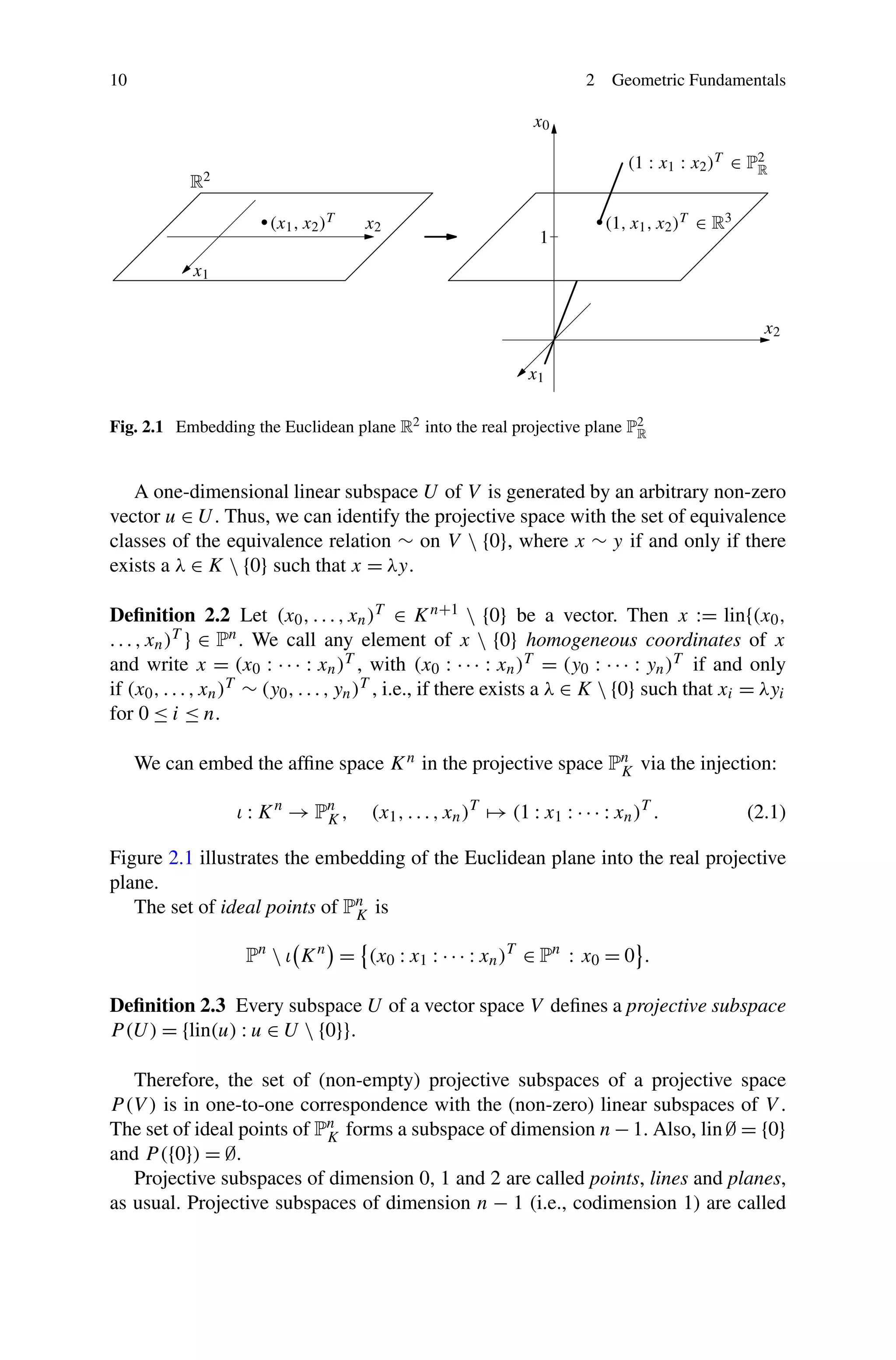
Chapter 2
Geometric Fundamentals


In this chapter we lay the geometric foundations that will serve as a basis for the
topics that we shall meet later. The statements of projective geometry, in contrast to
those of affine geometry, often allow a particularly simple formulation. The projec-
tive equivalence of polytopes and pointed polyhedra (Theorem 3.36) and Bézout’s
Theorem (Theorem 8.27) on the number of intersections of two algebraic curves in
the plane are good examples of this. We will also introduce the notion of convexity,
which is an irreplaceable concept in linear computational geometry.


2.1 Projective Spaces

The basic motivation behind the introduction of projective spaces comes from the
examination of two distinct lines in an arbitrary affine plane, for example the Eu-
clidean plane R2 . The lines either intersect or are parallel to one another. The funda-
mental idea of projective geometry is to extend the affine plane so that parallel lines
have an intersection point at “infinity”.
   For the remainder of this text, let K be an arbitrary field and for any subset A of
a vector space V , let lin A denote the linear hull of A. The cases K = R and K = C
are of primary interest in this book.

Definition 2.1
 (i) Let V be a finite dimensional vector space over K. The projective space P (V )
     induced by V is the set of one-dimensional subspaces of V . The dimension of
     P (V ) is defined as dim P (V ) = dim V − 1. The function which maps a vector
     v ∈ V  {0} to the one-dimensional linear subspace lin v is called the canonical
     projection.
(ii) For any natural number n, the set P (K n+1 ) is called the n-dimensional projec-
     tive space over K. We denote it by Pn and remove the lower index K if the
                                            K
     coordinate field is clear from the context.

M. Joswig, T. Theobald, Polyhedral and Algebraic Methods in Computational Geometry,   9
Universitext, DOI 10.1007/978-1-4471-4817-3_2,
© Springer-Verlag London 2013
10                                                                        2   Geometric Fundamentals


Fig. 2.1 Embedding the Euclidean plane R2 into the real projective plane P2
                                                                          R


   A one-dimensional linear subspace U of V is generated by an arbitrary non-zero
vector u ∈ U . Thus, we can identify the projective space with the set of equivalence
classes of the equivalence relation ∼ on V  {0}, where x ∼ y if and only if there
exists a λ ∈ K  {0} such that x = λy.

Definition 2.2 Let (x0 , . . . , xn )T ∈ K n+1  {0} be a vector. Then x := lin{(x0 ,
. . . , xn )T } ∈ Pn . We call any element of x  {0} homogeneous coordinates of x
and write x = (x0 : · · · : xn )T , with (x0 : · · · : xn )T = (y0 : · · · : yn )T if and only
if (x0 , . . . , xn )T ∼ (y0 , . . . , yn )T , i.e., if there exists a λ ∈ K  {0} such that xi = λyi
for 0 ≤ i ≤ n.

     We can embed the affine space K n in the projective space Pn via the injection:
                                                               K

                  ι : K n → Pn ,
                             K         (x1 , . . . , xn )T → (1 : x1 : · · · : xn )T .         (2.1)

Figure 2.1 illustrates the embedding of the Euclidean plane into the real projective
plane.
   The set of ideal points of Pn is
                               K

                    Pn  ι K n = (x0 : x1 : · · · : xn )T ∈ Pn : x0 = 0 .

Definition 2.3 Every subspace U of a vector space V defines a projective subspace
P (U ) = {lin(u) : u ∈ U  {0}}.

   Therefore, the set of (non-empty) projective subspaces of a projective space
P (V ) is in one-to-one correspondence with the (non-zero) linear subspaces of V .
The set of ideal points of Pn forms a subspace of dimension n − 1. Also, lin ∅ = {0}
                            K
and P ({0}) = ∅.
   Projective subspaces of dimension 0, 1 and 2 are called points, lines and planes,
as usual. Projective subspaces of dimension n − 1 (i.e., codimension 1) are called
2.1 Projective Spaces                                                                         11

hyperplanes. The embedding ι(U ) of a k-dimensional subspace U of K n produces
a k-dimensional projective subspace called the projective closure of U .

Example 2.4 Consider the projective plane P2 . The projective lines of this space
                                                 K
correspond to the two-dimensional subspaces of K 3 . Since the intersection of any
two distinct two-dimensional subspaces of K 3 is always one-dimensional, any two
distinct lines of the projective plane have a uniquely determined intersection point.
   Conversely, given any two distinct projective points there exists one unique pro-
jective line incident with both. This follows directly from the fact that the linear hull
of two distinct one-dimensional subspaces of a vector space is two-dimensional.

    The extension of the affine space K n to the projective space Pn simplifies many
                                                                   K
proofs by eliminating case distinctions. In the particularly interesting cases K = R
and K = C, the field K has a locally compact (and connected) topology, inducing
the product topology on K n . This topology has a natural extension to the point sets
Pn and Pn as a compactification. See Exercise 2.19.
  R       C
    Every hyperplane H in Pn can be expressed as the kernel of a non-trivial linear
                             K
form, that is, a K-linear map

            φ : K n+1 → K,       x = (x0 : · · · : xn )T → u0 x0 + · · · + un xn            (2.2)

where the coefficients u0 , . . . , un ∈ K are not all zero. The set of all K-linear forms
on K n+1 yields the dual space (K n+1 )∗ . Pointwise addition and scalar multiplica-
tion turns the dual space into a vector space over K. The map φ defined in (2.2) is
identified with the row vector u = (u0 , . . . , un ). Clearly, every hyperplane uniquely
defines the vector u = 0 up to a non-zero scalar and vice versa. In other words:
hyperplanes can also be expressed in terms of homogeneous coordinates, and we
simply write H = ker φ = [u0 : · · · : un ].
   The following proposition shows how hyperplanes can be expressed with the
help of the inner product

       ·, · : K n+1 × K n+1 → K,          x, y := x0 y0 + x1 y1 + · · · + xn yn             (2.3)

on K n+1 . For x ∈ K n+1 and u ∈ (K n+1 )∗ , we write

                                  u(x) = u · x = x, uT

where “·” denotes standard matrix multiplication.

Proposition 2.5 The projective point x = (x0 : · · · : xn )T lies in the projective hy-
perplane u = [u0 : · · · : un ] if and only if x, uT = 0.

Proof Notice that the condition x, uT = 0 makes sense in homogeneous coordi-
nates since it is homogeneous itself. The claim follows from the equation

    (λx0 , . . . , λxn )T , (μu0 , . . . , μun )T = λμ(x0 u0 + · · · + xn un ) = λμ x, uT

for every λ, μ ∈ K.
12                                                              2   Geometric Fundamentals

   At the end of the book, in Theorem 12.24, we will prove a far-reaching general-
ization of Proposition 2.5.

Example 2.6 As in Example 2.4, consider the affine plane K 2 and its projective clo-
sure, the projective plane P2 . We can use the homogeneous coordinates to represent
                            K
a projective line of P2 . For a, b, c ∈ K with (b, c) = (0, 0) let
                      K

                                  x
                           =        ∈ K 2 : a + bx + cy = 0
                                  y

be an arbitrary affine line. Then the projective line [a : b : c] is the projective closure
of . It contains exactly one extra projective point that is not the image of an affine
point of the embedding ι. This point is the ideal point of and has the homogeneous
coordinates (0 : c : −b).
    The homogeneous coordinates of every line of K 2 parallel to differ only in a,
their first coordinate (in the projective closure). Therefore, they share the same point
at infinity. All ideal points lie on the unique projective line [1 : 0 : 0], which is not
the projective closure of any affine line. This line is called the ideal line.
    Ideal points in the real projective plane P2 are often called points at infinity in
                                                R
the literature. The idea of two parallel lines “intersecting at infinity” means that the
projective closures of two parallel lines in R2 intersect at the same ideal point of P2 .
                                                                                        R


2.2 Projective Transformations
A linear transformation is a vector space automorphism, i.e., a bijective linear map
from a vector space to itself. Since projective spaces are defined in terms of vector
space quotients, linear transformations induce maps between the associated projec-
tive spaces.
   More precisely, let V be a finite dimensional K-vector space and f : V → V a
K-linear transformation. For v ∈ V  {0} and λ ∈ K we have f (λv) = λf (v) and
therefore f (lin(v)) = lin(f (v)). As f is bijective, non-zero vectors are mapped to
non-zero vectors. Hence f induces a projective transformation:

                    P (f ) : P (V ) → P (V ),    lin(v) → lin f (v) .

   For V = K n+1 , the map f is usually described by a matrix A ∈ GLn+1 K. We
will therefore use the notation [A] := P (f ) for projective transformations. Let
P (V ) be an n-dimensional projective space. A flag of length k is a sequence of
projective subspaces (U1 , . . . , Uk ) with U1 U2 · · · Uk . The maximal length
of a flag is n + 2. Every maximal flag begins with the empty set and ends with the
entire space P (V ).

Theorem 2.7 Let P (V ) be a finite dimensional projective space with two maximal
flags (U0 , . . . , Un+1 ) and (W0 , . . . , Wn+1 ). Then there exists a projective transfor-
mation π : P (V ) → P (V ) with π(Ui ) = Wi .
2.3 Convexity                                                                                    13

Proof Since the subspace Ui is strictly larger than Ui−1 , we can pick vectors u(i) ∈
Ui  Ui−1 for i ∈ {1, . . . , n + 1}. By construction u(i) is linearly independent of
u(1) , . . . , u(i−1) , and therefore (u(1) , . . . , u(n+1) ) is a basis of V . Similarly we obtain
a second basis (w (1) , . . . , w (n+1) ) from the second maximal flag (W0 , . . . , Wn+1 ).
   From linear algebra we know that there exists a unique invertible linear map
f : V → V that maps u(i) to w (i) for all i ∈ {1, . . . , n + 1}. Therefore π := P (f ) is
a projective transformation with the properties stated in the theorem.

   An equivalent formulation of the above statement is: The group of invertible
linear maps GL(V ) operates transitively on the maximal flags of P (V ).
   For a not necessarily maximal flag F = (V1 , . . . , Vk ) we call the strictly mono-
tone sequence of natural numbers (dimK V1 , . . . , dimK Vk ) the type of F .

Corollary 2.8 Let (U1 , . . . , Uk ) and (W1 , . . . , Wk ) be two flags of P (V ) with
the same types. Then there exists a projective transformation π on P (V ) with
π(Ui ) = Wi .

Proof Both (U1 , . . . , Uk ) and (W1 , . . . , Wk ) can be extended to maximal flags. Thus
the statement follows from Theorem 2.7.

   One may think that the uniqueness of the linear transformation f in the proof
of Theorem 2.7 implies the uniqueness of π = P (f ). Showing that this is generally
not true is the goal of the exercise below. First we clarify some terminology: A point
set M ⊆ Pn is called collinear if there exists a projective line that contains all points
of M. A quadruple (a (1) , a (2) , a (3) , a (4) ) of points of P2 is called a quadrangle if no
subset of three points is collinear.

Exercise 2.9 For any two quadrangles (a (1) , a (2) , a (3) , a (4) ) and (b(1) , b(2) ,
b(3) , b(4) ) there exists a projective transformation π of P2 with π(a (i) ) = b(i) for
1 ≤ i ≤ 4.

   An affine transformation is a projective transformation that maps ideal points to
ideal points.

Exercise 2.10 For every affine transformation π of Pn there exists a linear trans-
                                                    K
formation A ∈ GLn (K) and a vector v ∈ K n such that π(ι(x)) = ι(Ax + v) for all
x ∈ Kn.


2.3 Convexity

We begin by summarizing some notation from linear algebra to clarify the terminol-
ogy and concepts that we will use. As before, let K denote a field.
14                                                                  2   Geometric Fundamentals


Fig. 2.2 Affinely independent points (left) and affinely dependent points (middle and right) in the
Euclidean plane R2


Definition 2.11 Let A ⊆ K n . An affine combination of points in A is a linear
combination m λ(i) a (i) with m ≥ 1, λ(1) , . . . , λ(m) ∈ K, a (1) , . . . , a (m) ∈ A and
                i=1
   m
   i=1 λ = 1. The set of all affine combinations of A is called the affine hull of A
        (i)

or simply aff A. We call the points a (1) , . . . , a (m) ∈ K n affinely independent if they
generate an affine subspace of dimension m − 1.

    For example, the three points in the picture on the left hand side of Fig. 2.2 are
affinely independent and each set of four or more points in the real plane (as in
the middle and on the right hand side of Fig. 2.2) are affinely dependent. We set
aff ∅ = ∅ and dim ∅ = −1.
    The language of projective geometry allows us to describe linear algebra over
an arbitrary field in geometric terms. In the case of an ordered field like the real
numbers (and unlike C) we can further exploit the geometry to obtain results. For
the remaining part of this chapter, let K be the field R of real numbers.

Definition 2.12 Let A ⊆ Rn . A convex combination of A is an affine combination
  m    (i) (i) which additionally satisfies λ(1) , . . . , λ(m) ≥ 0. The set conv A of all
  i=1 λ a
convex combinations of A is called the convex hull of A. A set C ⊆ Rn is called
convex if it contains all convex combinations that can be obtained from it. The di-
mension of a convex set is the dimension of its affine hull.

   The empty set is convex by definition. The simplest non-trivial example of a
convex set is the closed interval [a, b] ⊆ R. It is one-dimensional and is the convex
hull of its end points. Analogously, for a, b ∈ Rn we define:

                  [a, b] := λa + (1 − λ)b : 0 ≤ λ ≤ 1 = conv{a, b}.

     See Fig. 2.3 for some examples.

Exercise 2.13 A set C ⊆ Rn is convex if and only if for every two points x, y ∈ C,
the segment [x, y] is contained in C.


2.3.1 Orientation of Affine Hyperplanes

For real numbers a0 , a1 , . . . , an with (a1 , . . . , an ) = 0 consider the affine hyper-
plane H = {x ∈ Rn : a0 + a1 x1 + · · · + an xn = 0}. Then [a0 : a1 : · · · : an ] are the
2.3 Convexity                                                                                  15


Fig. 2.3 Convex hulls of the points from Fig. 2.2


homogeneous coordinates of its projective closure. The complement Rn  H has two
connected components,
                   +
                  H◦ := x ∈ Rn : a0 + a1 x1 + · · · + an xn > 0                 and         (2.4)
                   −
                  H◦   := x ∈ R : a0 + a1 x1 + · · · + an xn < 0 .
                                    n
                                                                                            (2.5)

These components are called the open affine half-spaces defined by H , with H◦       +
      −
and H◦ attributed as positive and negative, respectively. The (closed) positive half-
space
                     H + := x ∈ Rn : a0 + a1 x1 + · · · + an xn ≥ 0
satisfies H + = H ∪ H◦ = Rn  H◦ . The opposite half-space H − is analogously
                      +                 −

defined. The vector (λa0 , λa1 , . . . , λan ) defines the same affine hyperplane H for
any λ = 0, however the roles of H + and H − are reversed when λ is negative. We
will let

             [a0 : a1 : · · · : an ]+ := x ∈ Rn : a0 + a1 x1 + · · · + an xn ≥ 0

and analogously define [a0 : a1 : · · · : an ]− . When we wish to distinguish which of
the two half-spaces defined by H is positive or negative, we will call [a0 : a1 : · · · :
an ] the oriented homogeneous coordinates of H .
    We often consider a given affine hyperplane H in Rn and use the notation H +
and H − without having first fixed a coordinate representation of H . This is simply a
notational device which enables us to differentiate between the two half-spaces; the
coordinates for H can always be chosen so that the notation is in accordance with
the above definition.
    The inner product introduced in (2.3) is the Euclidean scalar product on Rn . As
in Proposition 2.5 the sign of the scalar product

                            (1, x1 , . . . , xn )T , (a0 , a1 , . . . , an )T

denotes the half-space for [a0 : a1 : · · · : an ] in which the point (1, x1 , . . . , xn )T lies.


2.3.2 Separation Theorems

For M ⊆ Rn , we let int M denote the interior of M. That is, the set of points p ∈ M
for which there exists an -ball centered at p, completely contained in M. A set
16                                                             2   Geometric Fundamentals

is called open when int M = M and is closed if it is the complement of an open
set. The closure M of M is the smallest closed set in Rn containing M. The set
∂M := M  int M is the boundary of M. All of these terms are defined with respect
to the ambient space Rn .
    Some concepts from analysis are essential for the structure theory of convex sets.
The following statements rely on two core results which are proved in Appendix B.
Here, an affine hyperplane H is called a supporting hyperplane for a convex set
C ⊆ Rn if H ∩ C = ∅ and C is entirely contained in one of the closed affine half-
spaces determined by H .

Theorem 2.14 Let C be a closed and convex subset of Rn and p ∈ Rn  C an
exterior point. Then there exists an affine hyperplane H with C ⊆ H + and p ∈ H − ,
that meets neither C nor p.

     The next statement is a direct consequence of Theorem 2.14.

Corollary 2.15 Let C be a closed and convex subset of Rn . Then every point of the
boundary ∂C is contained in a supporting hyperplane.

   A convex set C ⊆ Rn is called full-dimensional if dim C = n. When C is not full
dimensional, it is often useful to use these topological concepts with respect to the
affine hull. The relative interior relint C of a convex set C consists of the interior
points of C interpreted as a subset of aff C. Analogously, the relative boundary of
C is the boundary of C as a subset of aff C.


2.4 Exercises
Exercise 2.16 Let P (V ) be a projective space. For every set S ⊆ V the set

                               T = lin{x} : x ∈ S  {0}

is a subset of P (V ) and for the subspace lin S generated by S, P (lin S) is a projective
subspace which we denote by T . Prove the dimension formula

                  dim U + dim W = dim U ∪ W            + dim(U ∩ W )

for two arbitrary projective subspaces U and W of P (V ).

Exercise 2.17 Let K be any field, and let A = (aij ) ∈ GLn+1 K. Show:
(a) If H is a projective hyperplane with homogeneous coordinates (h0 : h1 : · · · :
    hn ) then the image [A]H under the projective transformation [A] is the kernel
    of the linear form with coefficients (h0 , h1 , . . . , hn )A−1 .
(b) The projective transformation [A] acting on Pn is affine if and only if a12 =
                                                          K
    a13 = · · · = a1,n+1 = 0.
2.5 Remarks                                                                                 17

Exercise 2.18
(a) Every projective transformation on the real projective line P1 (apart from the
                                                                 R
    identity) has at most two fixed points.
(b) Every projective transformation on the complex projective line P1 (apart from
                                                                     C
    the identity) has at least one and at most two fixed points. (Explain why it is
    natural to talk about a double fixed point in the first case.)

   A projective space over a topological field has a natural topology that will be
discussed in the following exercise.

Exercise 2.19 Let K ∈ {R, C}. Show:
(a) The point set of a projective space Pn = Kn+1 /∼ is compact with respect to the
                                         K
    quotient topology.
(b) Every projective subspace of Pn , interpreted as a subset of the points of Pn , is
                                     K                                          K
    compact.

Exercise 2.20 Let K be a finite field with q elements.
(a) Show that the projective plane P2 has exactly N := q 2 + q + 1 points and
                                             K
    equally many lines.
(b) Denote by p (1) , . . . , p (N ) the points and by 1 , . . . , N the lines of P2 . Further-
                                                                                   K
    more, let A ∈ RN×N be the incidence matrix defined by

                                          1 if p (i) lies on   j,
                                 aij =
                                          0 otherwise.

    Compute the absolute value of the determinant of A. [Hint: Study the matrix
    A · AT .]

Exercise 2.21 (Carathéodory’s Theorem) If A ⊆ Rn and x ∈ conv A, then x can be
written as a convex combination of at most n + 1 points in A. [Hint: Since m ≥ n + 2
points are affinely dependent, every convex combination of m points in A can be
written as a convex combination of m − 1 points.]


2.5 Remarks
For further material on projective geometry, refer to the books of Beutelspacher and
Rosenbaum [13] and Richter-Gebert [88]. More detailed descriptions of convexity
can be found in Grünbaum [56, §2], Webster [98] or Gruber [55]. For basic topo-
logical concepts, see the books of Crossley [30] and Hatcher [58]. Although our
projective transformations are by definition always linearly induced, in other texts it
is common to extend this notion to include collineations induced by field automor-
phisms.
http://www.springer.com/978-1-4471-4816-6

Polyhedral and algebraic method in computational geometry

  • 1.
    Chapter 2 Geometric Fundamentals Inthis chapter we lay the geometric foundations that will serve as a basis for the topics that we shall meet later. The statements of projective geometry, in contrast to those of affine geometry, often allow a particularly simple formulation. The projec- tive equivalence of polytopes and pointed polyhedra (Theorem 3.36) and Bézout’s Theorem (Theorem 8.27) on the number of intersections of two algebraic curves in the plane are good examples of this. We will also introduce the notion of convexity, which is an irreplaceable concept in linear computational geometry. 2.1 Projective Spaces The basic motivation behind the introduction of projective spaces comes from the examination of two distinct lines in an arbitrary affine plane, for example the Eu- clidean plane R2 . The lines either intersect or are parallel to one another. The funda- mental idea of projective geometry is to extend the affine plane so that parallel lines have an intersection point at “infinity”. For the remainder of this text, let K be an arbitrary field and for any subset A of a vector space V , let lin A denote the linear hull of A. The cases K = R and K = C are of primary interest in this book. Definition 2.1 (i) Let V be a finite dimensional vector space over K. The projective space P (V ) induced by V is the set of one-dimensional subspaces of V . The dimension of P (V ) is defined as dim P (V ) = dim V − 1. The function which maps a vector v ∈ V {0} to the one-dimensional linear subspace lin v is called the canonical projection. (ii) For any natural number n, the set P (K n+1 ) is called the n-dimensional projec- tive space over K. We denote it by Pn and remove the lower index K if the K coordinate field is clear from the context. M. Joswig, T. Theobald, Polyhedral and Algebraic Methods in Computational Geometry, 9 Universitext, DOI 10.1007/978-1-4471-4817-3_2, © Springer-Verlag London 2013
  • 2.
    10 2 Geometric Fundamentals Fig. 2.1 Embedding the Euclidean plane R2 into the real projective plane P2 R A one-dimensional linear subspace U of V is generated by an arbitrary non-zero vector u ∈ U . Thus, we can identify the projective space with the set of equivalence classes of the equivalence relation ∼ on V {0}, where x ∼ y if and only if there exists a λ ∈ K {0} such that x = λy. Definition 2.2 Let (x0 , . . . , xn )T ∈ K n+1 {0} be a vector. Then x := lin{(x0 , . . . , xn )T } ∈ Pn . We call any element of x {0} homogeneous coordinates of x and write x = (x0 : · · · : xn )T , with (x0 : · · · : xn )T = (y0 : · · · : yn )T if and only if (x0 , . . . , xn )T ∼ (y0 , . . . , yn )T , i.e., if there exists a λ ∈ K {0} such that xi = λyi for 0 ≤ i ≤ n. We can embed the affine space K n in the projective space Pn via the injection: K ι : K n → Pn , K (x1 , . . . , xn )T → (1 : x1 : · · · : xn )T . (2.1) Figure 2.1 illustrates the embedding of the Euclidean plane into the real projective plane. The set of ideal points of Pn is K Pn ι K n = (x0 : x1 : · · · : xn )T ∈ Pn : x0 = 0 . Definition 2.3 Every subspace U of a vector space V defines a projective subspace P (U ) = {lin(u) : u ∈ U {0}}. Therefore, the set of (non-empty) projective subspaces of a projective space P (V ) is in one-to-one correspondence with the (non-zero) linear subspaces of V . The set of ideal points of Pn forms a subspace of dimension n − 1. Also, lin ∅ = {0} K and P ({0}) = ∅. Projective subspaces of dimension 0, 1 and 2 are called points, lines and planes, as usual. Projective subspaces of dimension n − 1 (i.e., codimension 1) are called
  • 3.
    2.1 Projective Spaces 11 hyperplanes. The embedding ι(U ) of a k-dimensional subspace U of K n produces a k-dimensional projective subspace called the projective closure of U . Example 2.4 Consider the projective plane P2 . The projective lines of this space K correspond to the two-dimensional subspaces of K 3 . Since the intersection of any two distinct two-dimensional subspaces of K 3 is always one-dimensional, any two distinct lines of the projective plane have a uniquely determined intersection point. Conversely, given any two distinct projective points there exists one unique pro- jective line incident with both. This follows directly from the fact that the linear hull of two distinct one-dimensional subspaces of a vector space is two-dimensional. The extension of the affine space K n to the projective space Pn simplifies many K proofs by eliminating case distinctions. In the particularly interesting cases K = R and K = C, the field K has a locally compact (and connected) topology, inducing the product topology on K n . This topology has a natural extension to the point sets Pn and Pn as a compactification. See Exercise 2.19. R C Every hyperplane H in Pn can be expressed as the kernel of a non-trivial linear K form, that is, a K-linear map φ : K n+1 → K, x = (x0 : · · · : xn )T → u0 x0 + · · · + un xn (2.2) where the coefficients u0 , . . . , un ∈ K are not all zero. The set of all K-linear forms on K n+1 yields the dual space (K n+1 )∗ . Pointwise addition and scalar multiplica- tion turns the dual space into a vector space over K. The map φ defined in (2.2) is identified with the row vector u = (u0 , . . . , un ). Clearly, every hyperplane uniquely defines the vector u = 0 up to a non-zero scalar and vice versa. In other words: hyperplanes can also be expressed in terms of homogeneous coordinates, and we simply write H = ker φ = [u0 : · · · : un ]. The following proposition shows how hyperplanes can be expressed with the help of the inner product ·, · : K n+1 × K n+1 → K, x, y := x0 y0 + x1 y1 + · · · + xn yn (2.3) on K n+1 . For x ∈ K n+1 and u ∈ (K n+1 )∗ , we write u(x) = u · x = x, uT where “·” denotes standard matrix multiplication. Proposition 2.5 The projective point x = (x0 : · · · : xn )T lies in the projective hy- perplane u = [u0 : · · · : un ] if and only if x, uT = 0. Proof Notice that the condition x, uT = 0 makes sense in homogeneous coordi- nates since it is homogeneous itself. The claim follows from the equation (λx0 , . . . , λxn )T , (μu0 , . . . , μun )T = λμ(x0 u0 + · · · + xn un ) = λμ x, uT for every λ, μ ∈ K.
  • 4.
    12 2 Geometric Fundamentals At the end of the book, in Theorem 12.24, we will prove a far-reaching general- ization of Proposition 2.5. Example 2.6 As in Example 2.4, consider the affine plane K 2 and its projective clo- sure, the projective plane P2 . We can use the homogeneous coordinates to represent K a projective line of P2 . For a, b, c ∈ K with (b, c) = (0, 0) let K x = ∈ K 2 : a + bx + cy = 0 y be an arbitrary affine line. Then the projective line [a : b : c] is the projective closure of . It contains exactly one extra projective point that is not the image of an affine point of the embedding ι. This point is the ideal point of and has the homogeneous coordinates (0 : c : −b). The homogeneous coordinates of every line of K 2 parallel to differ only in a, their first coordinate (in the projective closure). Therefore, they share the same point at infinity. All ideal points lie on the unique projective line [1 : 0 : 0], which is not the projective closure of any affine line. This line is called the ideal line. Ideal points in the real projective plane P2 are often called points at infinity in R the literature. The idea of two parallel lines “intersecting at infinity” means that the projective closures of two parallel lines in R2 intersect at the same ideal point of P2 . R 2.2 Projective Transformations A linear transformation is a vector space automorphism, i.e., a bijective linear map from a vector space to itself. Since projective spaces are defined in terms of vector space quotients, linear transformations induce maps between the associated projec- tive spaces. More precisely, let V be a finite dimensional K-vector space and f : V → V a K-linear transformation. For v ∈ V {0} and λ ∈ K we have f (λv) = λf (v) and therefore f (lin(v)) = lin(f (v)). As f is bijective, non-zero vectors are mapped to non-zero vectors. Hence f induces a projective transformation: P (f ) : P (V ) → P (V ), lin(v) → lin f (v) . For V = K n+1 , the map f is usually described by a matrix A ∈ GLn+1 K. We will therefore use the notation [A] := P (f ) for projective transformations. Let P (V ) be an n-dimensional projective space. A flag of length k is a sequence of projective subspaces (U1 , . . . , Uk ) with U1 U2 · · · Uk . The maximal length of a flag is n + 2. Every maximal flag begins with the empty set and ends with the entire space P (V ). Theorem 2.7 Let P (V ) be a finite dimensional projective space with two maximal flags (U0 , . . . , Un+1 ) and (W0 , . . . , Wn+1 ). Then there exists a projective transfor- mation π : P (V ) → P (V ) with π(Ui ) = Wi .
  • 5.
    2.3 Convexity 13 Proof Since the subspace Ui is strictly larger than Ui−1 , we can pick vectors u(i) ∈ Ui Ui−1 for i ∈ {1, . . . , n + 1}. By construction u(i) is linearly independent of u(1) , . . . , u(i−1) , and therefore (u(1) , . . . , u(n+1) ) is a basis of V . Similarly we obtain a second basis (w (1) , . . . , w (n+1) ) from the second maximal flag (W0 , . . . , Wn+1 ). From linear algebra we know that there exists a unique invertible linear map f : V → V that maps u(i) to w (i) for all i ∈ {1, . . . , n + 1}. Therefore π := P (f ) is a projective transformation with the properties stated in the theorem. An equivalent formulation of the above statement is: The group of invertible linear maps GL(V ) operates transitively on the maximal flags of P (V ). For a not necessarily maximal flag F = (V1 , . . . , Vk ) we call the strictly mono- tone sequence of natural numbers (dimK V1 , . . . , dimK Vk ) the type of F . Corollary 2.8 Let (U1 , . . . , Uk ) and (W1 , . . . , Wk ) be two flags of P (V ) with the same types. Then there exists a projective transformation π on P (V ) with π(Ui ) = Wi . Proof Both (U1 , . . . , Uk ) and (W1 , . . . , Wk ) can be extended to maximal flags. Thus the statement follows from Theorem 2.7. One may think that the uniqueness of the linear transformation f in the proof of Theorem 2.7 implies the uniqueness of π = P (f ). Showing that this is generally not true is the goal of the exercise below. First we clarify some terminology: A point set M ⊆ Pn is called collinear if there exists a projective line that contains all points of M. A quadruple (a (1) , a (2) , a (3) , a (4) ) of points of P2 is called a quadrangle if no subset of three points is collinear. Exercise 2.9 For any two quadrangles (a (1) , a (2) , a (3) , a (4) ) and (b(1) , b(2) , b(3) , b(4) ) there exists a projective transformation π of P2 with π(a (i) ) = b(i) for 1 ≤ i ≤ 4. An affine transformation is a projective transformation that maps ideal points to ideal points. Exercise 2.10 For every affine transformation π of Pn there exists a linear trans- K formation A ∈ GLn (K) and a vector v ∈ K n such that π(ι(x)) = ι(Ax + v) for all x ∈ Kn. 2.3 Convexity We begin by summarizing some notation from linear algebra to clarify the terminol- ogy and concepts that we will use. As before, let K denote a field.
  • 6.
    14 2 Geometric Fundamentals Fig. 2.2 Affinely independent points (left) and affinely dependent points (middle and right) in the Euclidean plane R2 Definition 2.11 Let A ⊆ K n . An affine combination of points in A is a linear combination m λ(i) a (i) with m ≥ 1, λ(1) , . . . , λ(m) ∈ K, a (1) , . . . , a (m) ∈ A and i=1 m i=1 λ = 1. The set of all affine combinations of A is called the affine hull of A (i) or simply aff A. We call the points a (1) , . . . , a (m) ∈ K n affinely independent if they generate an affine subspace of dimension m − 1. For example, the three points in the picture on the left hand side of Fig. 2.2 are affinely independent and each set of four or more points in the real plane (as in the middle and on the right hand side of Fig. 2.2) are affinely dependent. We set aff ∅ = ∅ and dim ∅ = −1. The language of projective geometry allows us to describe linear algebra over an arbitrary field in geometric terms. In the case of an ordered field like the real numbers (and unlike C) we can further exploit the geometry to obtain results. For the remaining part of this chapter, let K be the field R of real numbers. Definition 2.12 Let A ⊆ Rn . A convex combination of A is an affine combination m (i) (i) which additionally satisfies λ(1) , . . . , λ(m) ≥ 0. The set conv A of all i=1 λ a convex combinations of A is called the convex hull of A. A set C ⊆ Rn is called convex if it contains all convex combinations that can be obtained from it. The di- mension of a convex set is the dimension of its affine hull. The empty set is convex by definition. The simplest non-trivial example of a convex set is the closed interval [a, b] ⊆ R. It is one-dimensional and is the convex hull of its end points. Analogously, for a, b ∈ Rn we define: [a, b] := λa + (1 − λ)b : 0 ≤ λ ≤ 1 = conv{a, b}. See Fig. 2.3 for some examples. Exercise 2.13 A set C ⊆ Rn is convex if and only if for every two points x, y ∈ C, the segment [x, y] is contained in C. 2.3.1 Orientation of Affine Hyperplanes For real numbers a0 , a1 , . . . , an with (a1 , . . . , an ) = 0 consider the affine hyper- plane H = {x ∈ Rn : a0 + a1 x1 + · · · + an xn = 0}. Then [a0 : a1 : · · · : an ] are the
  • 7.
    2.3 Convexity 15 Fig. 2.3 Convex hulls of the points from Fig. 2.2 homogeneous coordinates of its projective closure. The complement Rn H has two connected components, + H◦ := x ∈ Rn : a0 + a1 x1 + · · · + an xn > 0 and (2.4) − H◦ := x ∈ R : a0 + a1 x1 + · · · + an xn < 0 . n (2.5) These components are called the open affine half-spaces defined by H , with H◦ + − and H◦ attributed as positive and negative, respectively. The (closed) positive half- space H + := x ∈ Rn : a0 + a1 x1 + · · · + an xn ≥ 0 satisfies H + = H ∪ H◦ = Rn H◦ . The opposite half-space H − is analogously + − defined. The vector (λa0 , λa1 , . . . , λan ) defines the same affine hyperplane H for any λ = 0, however the roles of H + and H − are reversed when λ is negative. We will let [a0 : a1 : · · · : an ]+ := x ∈ Rn : a0 + a1 x1 + · · · + an xn ≥ 0 and analogously define [a0 : a1 : · · · : an ]− . When we wish to distinguish which of the two half-spaces defined by H is positive or negative, we will call [a0 : a1 : · · · : an ] the oriented homogeneous coordinates of H . We often consider a given affine hyperplane H in Rn and use the notation H + and H − without having first fixed a coordinate representation of H . This is simply a notational device which enables us to differentiate between the two half-spaces; the coordinates for H can always be chosen so that the notation is in accordance with the above definition. The inner product introduced in (2.3) is the Euclidean scalar product on Rn . As in Proposition 2.5 the sign of the scalar product (1, x1 , . . . , xn )T , (a0 , a1 , . . . , an )T denotes the half-space for [a0 : a1 : · · · : an ] in which the point (1, x1 , . . . , xn )T lies. 2.3.2 Separation Theorems For M ⊆ Rn , we let int M denote the interior of M. That is, the set of points p ∈ M for which there exists an -ball centered at p, completely contained in M. A set
  • 8.
    16 2 Geometric Fundamentals is called open when int M = M and is closed if it is the complement of an open set. The closure M of M is the smallest closed set in Rn containing M. The set ∂M := M int M is the boundary of M. All of these terms are defined with respect to the ambient space Rn . Some concepts from analysis are essential for the structure theory of convex sets. The following statements rely on two core results which are proved in Appendix B. Here, an affine hyperplane H is called a supporting hyperplane for a convex set C ⊆ Rn if H ∩ C = ∅ and C is entirely contained in one of the closed affine half- spaces determined by H . Theorem 2.14 Let C be a closed and convex subset of Rn and p ∈ Rn C an exterior point. Then there exists an affine hyperplane H with C ⊆ H + and p ∈ H − , that meets neither C nor p. The next statement is a direct consequence of Theorem 2.14. Corollary 2.15 Let C be a closed and convex subset of Rn . Then every point of the boundary ∂C is contained in a supporting hyperplane. A convex set C ⊆ Rn is called full-dimensional if dim C = n. When C is not full dimensional, it is often useful to use these topological concepts with respect to the affine hull. The relative interior relint C of a convex set C consists of the interior points of C interpreted as a subset of aff C. Analogously, the relative boundary of C is the boundary of C as a subset of aff C. 2.4 Exercises Exercise 2.16 Let P (V ) be a projective space. For every set S ⊆ V the set T = lin{x} : x ∈ S {0} is a subset of P (V ) and for the subspace lin S generated by S, P (lin S) is a projective subspace which we denote by T . Prove the dimension formula dim U + dim W = dim U ∪ W + dim(U ∩ W ) for two arbitrary projective subspaces U and W of P (V ). Exercise 2.17 Let K be any field, and let A = (aij ) ∈ GLn+1 K. Show: (a) If H is a projective hyperplane with homogeneous coordinates (h0 : h1 : · · · : hn ) then the image [A]H under the projective transformation [A] is the kernel of the linear form with coefficients (h0 , h1 , . . . , hn )A−1 . (b) The projective transformation [A] acting on Pn is affine if and only if a12 = K a13 = · · · = a1,n+1 = 0.
  • 9.
    2.5 Remarks 17 Exercise 2.18 (a) Every projective transformation on the real projective line P1 (apart from the R identity) has at most two fixed points. (b) Every projective transformation on the complex projective line P1 (apart from C the identity) has at least one and at most two fixed points. (Explain why it is natural to talk about a double fixed point in the first case.) A projective space over a topological field has a natural topology that will be discussed in the following exercise. Exercise 2.19 Let K ∈ {R, C}. Show: (a) The point set of a projective space Pn = Kn+1 /∼ is compact with respect to the K quotient topology. (b) Every projective subspace of Pn , interpreted as a subset of the points of Pn , is K K compact. Exercise 2.20 Let K be a finite field with q elements. (a) Show that the projective plane P2 has exactly N := q 2 + q + 1 points and K equally many lines. (b) Denote by p (1) , . . . , p (N ) the points and by 1 , . . . , N the lines of P2 . Further- K more, let A ∈ RN×N be the incidence matrix defined by 1 if p (i) lies on j, aij = 0 otherwise. Compute the absolute value of the determinant of A. [Hint: Study the matrix A · AT .] Exercise 2.21 (Carathéodory’s Theorem) If A ⊆ Rn and x ∈ conv A, then x can be written as a convex combination of at most n + 1 points in A. [Hint: Since m ≥ n + 2 points are affinely dependent, every convex combination of m points in A can be written as a convex combination of m − 1 points.] 2.5 Remarks For further material on projective geometry, refer to the books of Beutelspacher and Rosenbaum [13] and Richter-Gebert [88]. More detailed descriptions of convexity can be found in Grünbaum [56, §2], Webster [98] or Gruber [55]. For basic topo- logical concepts, see the books of Crossley [30] and Hatcher [58]. Although our projective transformations are by definition always linearly induced, in other texts it is common to extend this notion to include collineations induced by field automor- phisms.
  • 10.