This document discusses various aspects of signal propagation including:
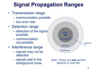
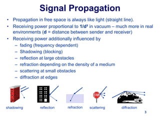
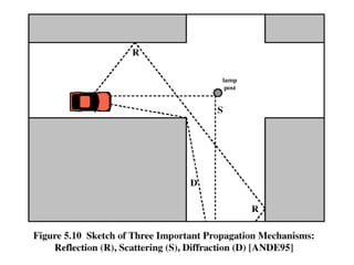
1. It defines transmission, detection, and interference ranges for wireless signals. The receiving power decreases with distance and is influenced by factors like fading, shadowing, reflection, refraction, scattering, and diffraction.
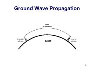
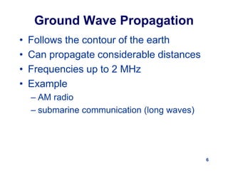
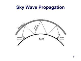
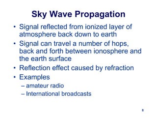
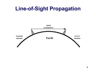
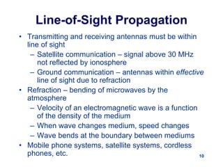
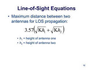
2. It describes three main propagation modes - ground-wave propagation below 2MHz, sky-wave propagation between 2-30MHz using ionospheric reflection, and line-of-sight propagation above 30MHz requiring a direct path.
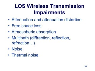
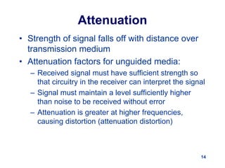
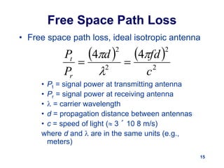
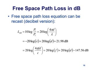
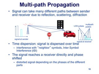
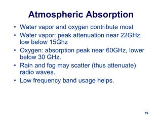
3. Factors that impair line-of-sight wireless transmission include attenuation, free space loss, atmospheric absorption, multipath effects, noise, and mobility-induced fading. Techniques like error correction and