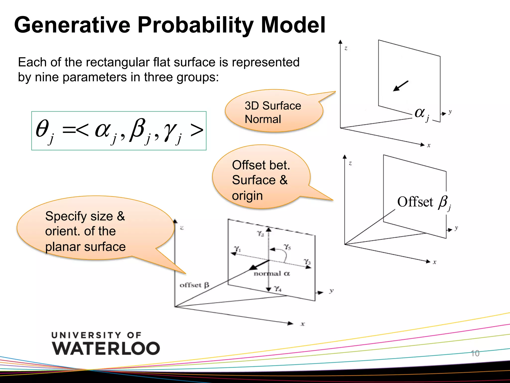
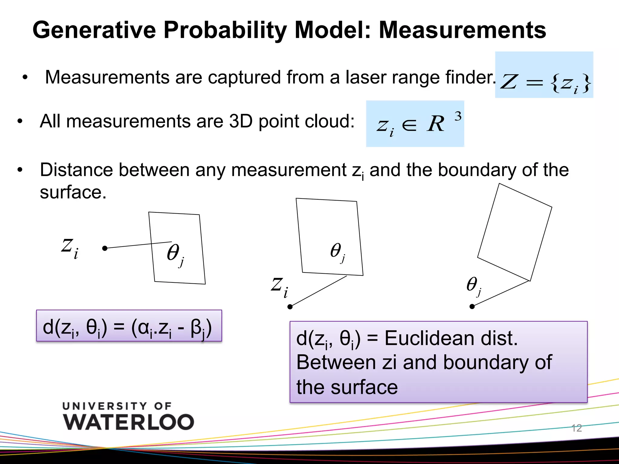
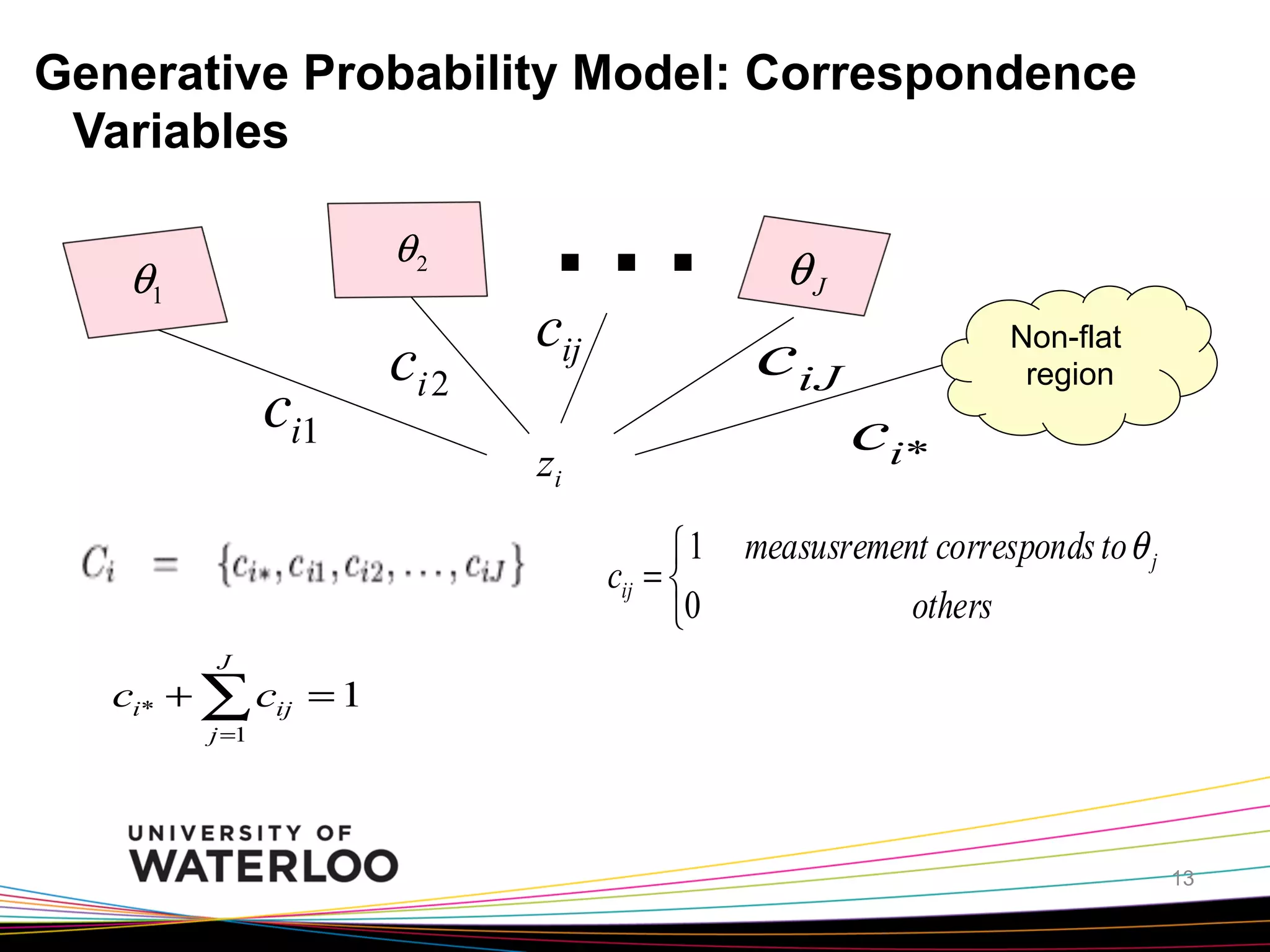
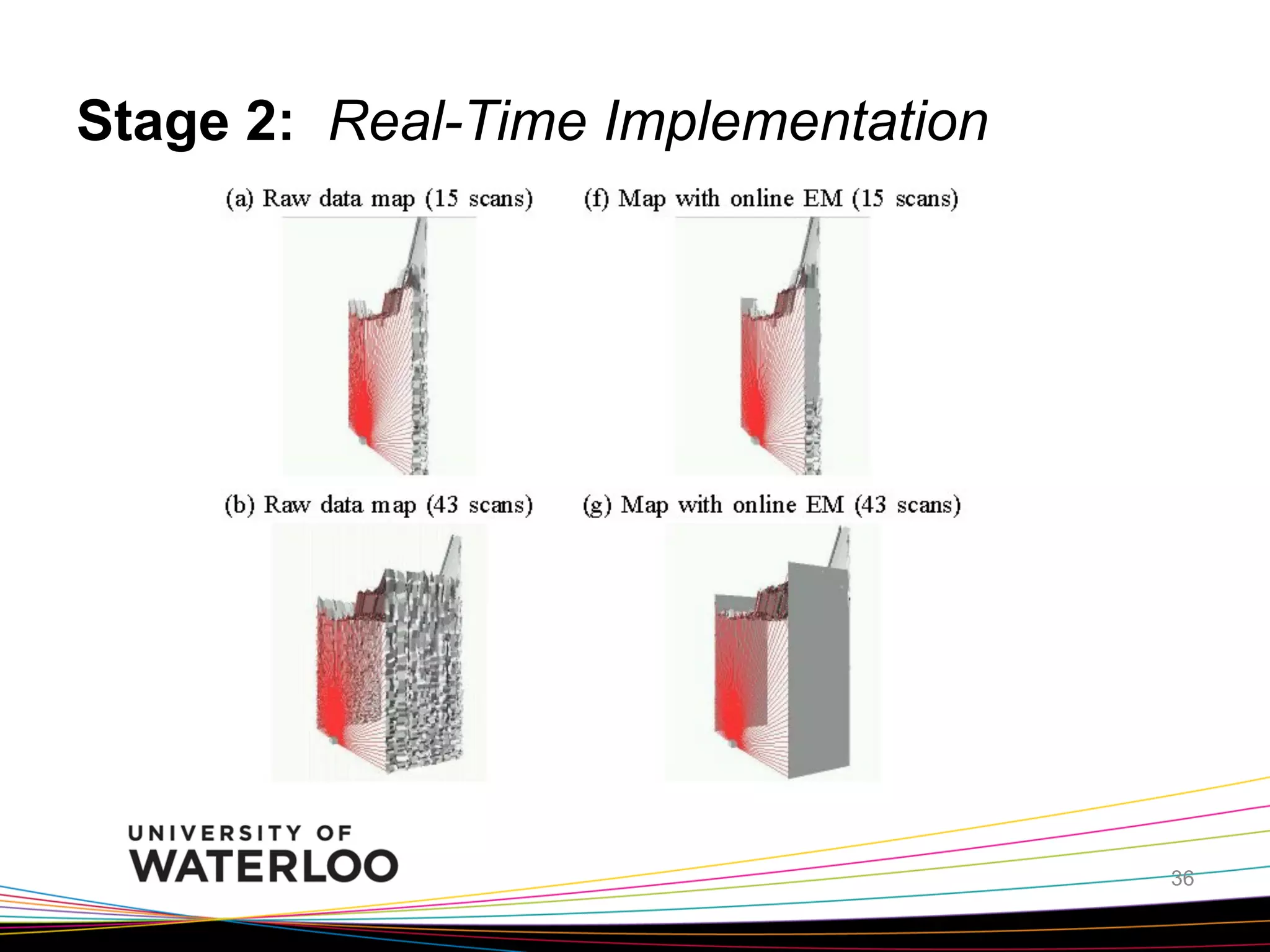
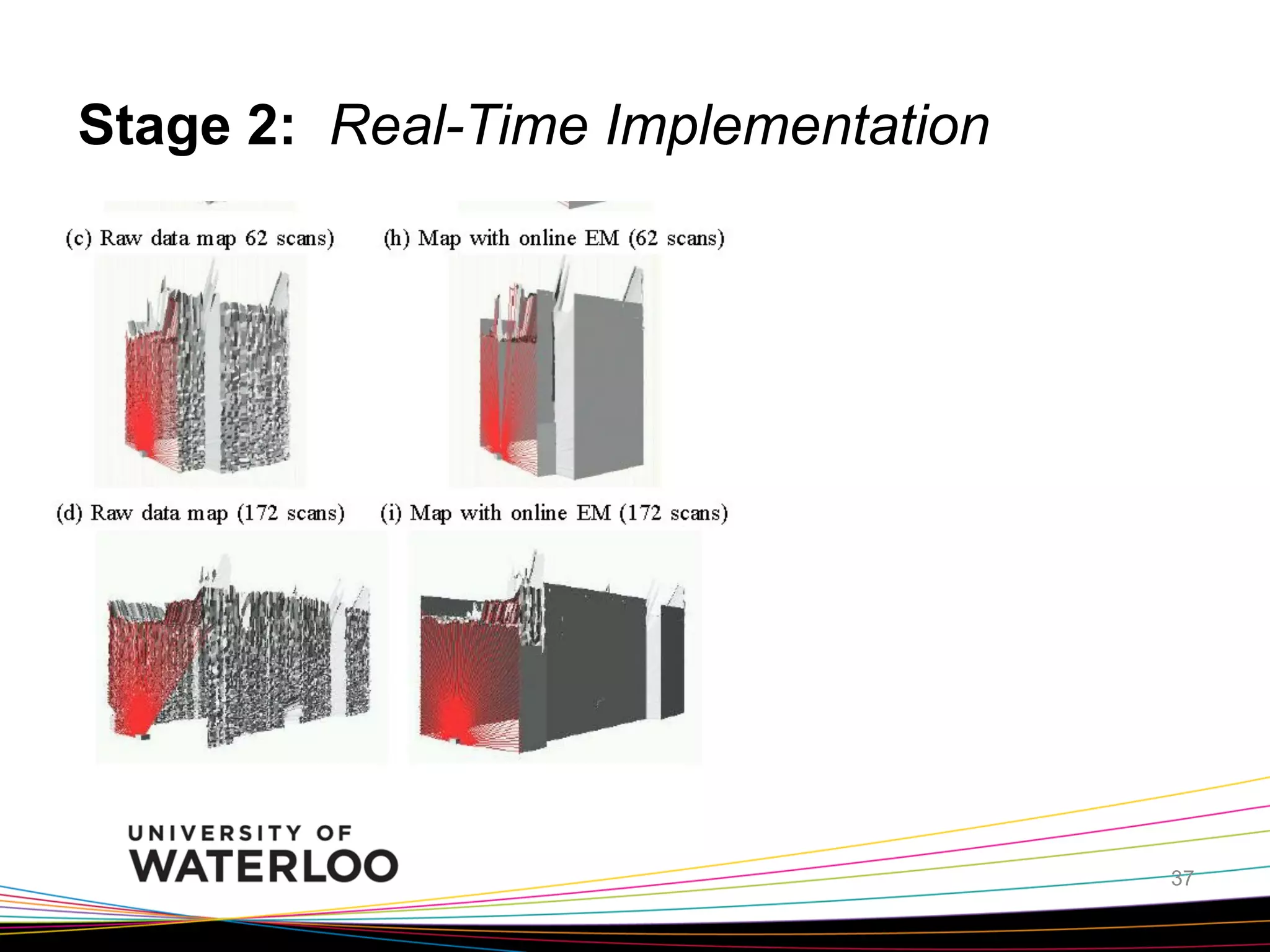
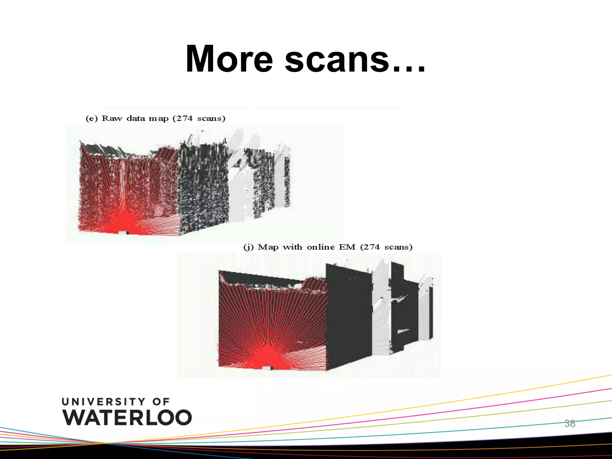
This document summarizes a probabilistic algorithm for online 3D mobile robot mapping presented by Noha Quan Ravi. The algorithm uses an online Expectation-Maximization approach to build 3D maps from laser rangefinder and camera sensor data in real-time. It models the environment as planar surfaces and represents each surface with nine parameters. The algorithm iterates between estimating surface correspondences to measurements (E-step) and re-estimating the surface parameters (M-step). It processes a constant number of new measurements at each time step to allow real-time mapping performance as the robot moves through its environment. Experimental results demonstrate it can successfully build 3D maps of indoor environments in real-time.

1. Probabilistic Algorithms for
Mobile Robot Mapping
Presented by: Noha Quan Ravi

2. Based on the paper
A Real-Time Algorithm for Mobile Robot Mapping
With Applications to Multi-Robot and 3D Mapping
Best paper award at 2000 IEEE International
Conference on Robotics and Automation (~1,100
submissions)
By: Sebastian Thrun et. al.
2

3. Robot Mapping…
• Robot Mapping aims is to build a
map of the physical environment of
the robot
• Maps are utilized by mobile robots
for their operations.
• Mapping: generating models of
robot environments from sensor
data.
• Probabilistic methods have
recently proved very effective.
• Wide variety of sensors are used,
with different characteristics (e.g.
sonar, laser, IR, cameras, GPS)
3

4. Robot Mapping Applications
The Nursebot Initiative
Roomba – Autonomic
robotic vacuum cleaners
Serviceroboter
Museum Tour-Guide Robots

5. video
5

6. Problem
q Building an Online 3D Indoor Robot map.
• Challenges:
1. Measurement Noise.
2. High dimensionality of the mapped
entities.(2D Vs. 3D).
3. Dynamic environment.
4. Data association (correspondence) problem.
5. Robotic Localization.
(SLAM: Simultaneous Localization & Mapping)
6

7. Related Work
Ø Focused on building maps in 2D from sensor
measurements.
- Line extraction from a single scan.
Ø 3D system models proposed by Roth* doesn’t
consider uncertainty of individual measurements
when generating the 3D model.
* G. Roth and R. Wibowo, “A fast algorithm for making mesh-models
from multiple-view range data,” in Proceedings of the DND/CSA
Robotics and Knowledge Based Systems Workshop, 1995.
7

8. Methodology
• Propose an algorithm “Online EM” for 3D models for indoor
mappings that works in real time.
• Measurements are captured using laser range finder and
panoramic camera.
• Evaluation of the proposed algorithm via real-time
implementation in several different buildings.
• Assumptions:
Ø prior knowledge : the shape of basic building elements.
Ø Robot pose is given.
8

9. Agenda
9

10. Generative Probability Model
Each of the rectangular flat surface is represented
by nine parameters in three groups:
θ j =< α j , β j , γ j >
3D Surface
Normal
Offset bet.
Surface &
origin
Specify size &
orient. of the
planar surface
!j
Offset β j
10

11. Generative Probability Model: World Model
• Two types of surfaces:
θ1
θ2
…
θJ
θ = {θ1 ,θ 2 ...,θ J }
Flat Surfaces
Non-flat region
11

12. Generative Probability Model: Measurements
• Measurements are captured from a laser range finder. Z = {z }
i
• All measurements are 3D point cloud:
zi ∈ R
3
• Distance between any measurement zi and the boundary of the
surface.
zi
θj
d(zi, θi) = (αi.zi - βj)
θj
zi
θj
d(zi, θi) = Euclidean dist.
zi
Between zi and boundary of
the surface
12

13. Generative Probability Model: Correspondence
Variables
θ2
θ1
ci1
ci 2
…
cij
θJ
ciJ
zi
⎧1
cij = ⎨
⎩0
Non-flat
region
ci*
measusrement corresponds to θ j
others
J
ci* + ∑ cij = 1
j =1
13

14. Measurement Model
Probabilistic generative model of the measurements given the world.
P( zi | Ci, θ )
14

15. Agenda
15

16. Error Distribution
A. For flat surfaces (Normal distribution)
p( zi | cij = 1,θ ) =
1
2πσ
2
e
2
1 d ( zi ,θ j )
−
2
σ2
B. For non-flat surfaces (Uniform distribution)
⎧1 / z max ,
p( zi | cij = 1, θ ) = ⎨
⎩ 0,
1
z max
=
1
2πσ
2
e
if 0 ≤ zi ≤ z max
otherwise
1
z 2 max
− log
2
2πσ 2
16

17. The Log-Likelihood Function
• Sensor Model: Conditional probability
p( zi | Ci ,θ ) =
1
2πσ 2
e
1
z 2 ma x
− [ ci* log
+
2
2
2πσ
∑ j cij
d 2 ( zi ,θ j )
σ
2
]
• Sensor Model: Joint probability
p( zi , Ci | θ ) =
1
( J + 1) 2πσ 2
e
1
z 2 max
− [ ci* log
+
2
2
2πσ
∑ j cij
d 2 ( zi ,θ j )
σ
2
]
17

18. The Expectation of the log likelihood
• Assuming independence in measurement noise:
p( Z , C | θ )
=∏
i
1
( J + 1) 2πσ
2
e
1
z 2 max
− [ ci* log
+
2
2πσ 2
∑ j cij
d 2 ( zi ,θ j )
σ2
]
• EM: take the log likelihood (take the log of the above equation)
EC = [log p ( Z , C | θ ) | Z , θ ]
⎡
1
1
z 2 max
∑ ⎢log ( J + 1) 2πσ 2 − 2 E[ci* | zi ,θ ] log 2πσ 2
i ⎢
⎣
d 2 ( zi , θ j ) ⎤
1
− ∑ j E[cij | zi , θ ]
⎥
2
σ2 ⎥
⎦
18

19. Agenda
19

20. EM Algorithm: offline
• A popular method for optimization
• Uses hill climbing in likelihood space.
• Used for problems with latent variables.
z
• Input: measurement i,
the 3D points
1
• Output:
[ n +1]
< α [ n+1] , β [ n+1] , γ [ n+1] >
A map θ
which maximize the expectation log likelihood
over correspondences C
• EM is an iterative process. Each iteration
includes two steps: E-step and M-step.
θ
...
θ2
θJ
Non-flat
region

21. EM Algorithm: offline
A. The E-Step
- Initialize θ [0] = A random map
- Calculate the expectations of the unknown
correspondences for the current map θ [n] .
[
eijn ] = E[cij | zi ,θ [ n ] ] = p(cij | zi ,θ [ n ] )
p( zi | cij ,θ ) p(cij | θ )
[n]
=
[n]
p ( zi | θ [ n ] )
e
=
e
2
z max
2
1
− log
2 2πσ
2
1 d ( zi |θ j )
−
2 σ2
+ ∑k e
−
2
1 d ( zi |θ k )
2 σ2
ei[*n ] = E[ci* | zi ,θ [ n ] ] = p(cij | zi ,θ [ n ] )
p( zi | ci* ,θ [ n ] ) p(ci* | θ [ n ] )
=
p ( zi | θ [ n ] )
e
=
e
2
z max
1
− log
2 2πσ 2
z2
1
− log max2
2 2πσ
+ ∑k e
1 d 2 ( zi |θ k )
−
2 σ2
21

22. EM Algorithm: offline (cont.)
B. The M-Step
• Goal: Maximize the expectation of the log likelihood where
the expectation is taken over all the correspondences C.
EC = [log p(Z , C | θ ) | Z ,θ ]
⎡
1
1
z 2 max
∑ ⎢log ( J + 1) 2πσ 2 − 2 E[ci* | zi ,θ ] log 2πσ 2
i ⎢
⎣
d 2 ( zi , θ j ) ⎤
1
− ∑ j E[cij | zi ,θ ]
⎥
2
σ2 ⎥
⎦
The quadratic optimization problem is solved via Lagrange multipliers.
22

23. Agenda
23

24. Online EM
• Offline EM Limitations
• 1. Require all the measurements Z as input
• 2. Access every measurement zi and every
θ j per iteration d 2 ( zi ,θ j )
model
• 3. Computation grows as dataset grows
• Solution: Online EM
24

25. Online EM
• Key idea:
• Each time interval, constant number of new
range measurements arrive
• Advantages:
• 1. Acquire compact 3-D models in real time
• 2. Limited number of measurements as input
• 3. Constant time per iteration
25

26. Online EM (Online E-Step)
• Constant number of measurements
• 1.New arrival measurements
• 2. Old measurements
– At the boundary of two surface models
– Unexplained by any existing surface models
• Counter
• 1. Record E-step calculation times
• 2. Freeze when achieve a threshold
26

27. Online EM (Online M-Step)
• Goal:
• Re-estimate the parameters of flat surface model
in constant time
• Control:
• The number of flat surfaces
• The number of measurements
27

28. Online EM (Online M-Step)
• Control the number of flat surfaces :
• Active flat surface model only
• Definition of “active”:
• A surface is active at time i if the E-step
executed at that time changed the ML
correspondence to or away from the surface for
any of the updated measurement.
28

29. Online EM
(Model Selection)
q Add new models
Ø New measurements not “explained” by existing surface
models
Ø “explained”:
likelihood > threshold
Ø not “explained”: seed for new surface
q Remove models
Ø The surface model is not supported by sufficient
measurements
29

30. Agenda
30

31. Experimental Results
• Two stages
– Offline EM algorithm.
168,120 range measurements
3,270 camera images,
extracted 3,220,950 pixels
Two minutes
– Real time online version of our approach
• Different buildings
• Three examples in paper (One presented here)
31

32. Stage 1: Offline EM
Map without the texture
superimposed.
32

33. Map with Texture vs. EM algorithm
33

34. Non-planar surfaces
Non-planer region was
not mapped to any of the
surfaces (!)
34

35. Number of surfaces -
J
Every 20 steps surfaces are
restarted.
500 iterations J settles down to
8.76+/- 1.46 (95.5+-0.006% )
20 minutes for 2000 iterations.
35

36. Stage 2: Real-Time Implementation
36

37. Stage 2: Real-Time Implementation
37

38. More scans…
38

39. Agenda
39

40. Conclusion - Main Contributions
• Convert EM from offline to online
• Compact & accurate computations.
• 3D mapping instead of 2D mapping
• Handles surfaces in arbitrary orientations.
40

41. Conclusion - Critical Analysis
• Models are visually realistic but not geometrically
accurate.
• Not best in occluded/unstructured environments.
• Test data has hallways with no furniture/occlusions.
• Starts with Assumption that surfaces as flat.
• Quality of images is not good enough for eye-inhand. just suffices robot movement.
41

42. Future Work
• Can be used for representing more complex
models.
• Outdoor mapping
• Use EM to perform SLAM.
42

43. Questions ?
43