Camera calibration is an important problem in 3D computer vision. The problem of determining the camera parameters has been studied extensively. However the algorithms for determining the required correspondences are either semi-automatic (i.e. they require user interaction) or they involve difficult to implement custom algorithms. We present a robust algorithm for detecting the corners of a calibration grid and assigning the correct correspondences for calibration . The solution is based on generic image processing operations so that it can be implemented quickly. The algorithm is limited to distortion-free cameras but it could potentially be extended to deal with camera distortion as well. We also present a corner detector based on steerable filters. The corner detector is particularly suited for the problem of detecting the corners of a calibration grid. - See more at: http://figshare.com/articles/Using_Generic_Image_Processing_Operations_to_Detect_a_Calibration_Grid/696880#sthash.EG8dWyTH.dpuf

1. Using Generic Image Processing Operations to
Detect a Calibration Grid
J. Wedekind∗
and J. Penders∗
and M. Howarth∗
and A. J. Lockwood+
and K. Sasada!
∗
Materials and Engineering Research Institute, Sheffield Hallam University, Pond Street, Sheffield S1 1WB, United Kingdom
+
Department of Engineering Materials, The University of Sheffield, Mappin Street, Sheffield S1 3JD, United Kingdom
!
Department of Creative Informatics, The University of Tokyo, 7-3-1 Hongo, Bunkyo-ku, Tokyo 113-8656, Japan
May 2, 2013
Abstract
Camera calibration is an important problem in 3D computer vision. The
problem of determining the camera parameters has been studied extensively.
However the algorithms for determining the required correspondences are
either semi-automatic (i.e. they require user interaction) or they involve dif-
ficult to implement custom algorithms.
We present a robust algorithm for detecting the corners of a calibration
grid and assigning the correct correspondences for calibration . The solu-
tion is based on generic image processing operations so that it can be im-
plemented quickly. The algorithm is limited to distortion-free cameras but it
could potentially be extended to deal with camera distortion as well.
We also present a corner detector based on steerable filters. The corner
detector is particularly suited for the problem of detecting the corners of a
calibration grid.
Key Words: computer vision, 3D and stereo, algorithms, calibration
1 Introduction
Camera calibration is a fundamental requirement for 3D computer vision. Deter-
mining the camera parameters is crucial for 3D mapping and object recognition.
There are methods for auto-calibration using a video from a static scene (e.g. see
[9]). However if possible, off-line calibration using a calibration object is used,
because it is more robust and easier to implement.
1

2. 2
± ±
(m1, m1)
(m2, m2)
(m3, m3)
. . .
±H
Figure 1: The different stages of determining a planar homography
The problem of estimating the camera parameters given some calibration data
has been studied extensively ([12], [1], [15]). However the solutions for determin-
ing the initial correspondences are either semi-automatic (i.e. they require user
intraction) or they involve difficult to implement custom algorithms.
This publication presents
• a filter for locating chequerboard-like corners and
• an algorithm for identifying and ordering the corners of the calibration grid
The algorithm is based on standard image processing operations and is thus
easy to implement. The corner detector does not suffer from the problem of pro-
ducing duplicate corners. The algorithm for detecting the calibration grid is robust
even in the presence of background clutter.
This paper is organised as follows. Section 2 gives an overview of the state of
the art. Section 3 presents a corner detector based on steerable patterns. Section 4
presents a novel algorithm for robust detection of the corners of a calibration grid.
Zhengyou Zhang’s method for determining the planar homography [15] is briefly
introduced in Section 5. Section 6 explains a simple special case of Zhengyou
Zhang’s method for determining the camera intrinsic matrix. Results and conclu-
sions are given in Section 7 and 8.
2 Calibration using Chequerboard Pattern
Usually the camera is calibrated by taking sequence of pictures showing a chequer-
board pattern of known size. The chequerboard is a simple repetitive pattern, i.e.
knowing the width, height, and the size of each square, one can infer the 2D planar
coordinate of each corner. The correspondences between picture coordinates and
real-world coordinates are used to determine the parameters of the camera (also
see Figure 1). The calibration process is as follows
• The camera takes a picture of the calibration grid which has corners at the
known positions m1, m2, . . .

3. 3
Figure 2: Harris-Stephens corner detection followed by non-maxima suppression.
The corner detector sometimes produces duplicate corners
• The coordinates m1, m2, . . . of the corners in the camera image are deter-
mined
• The correspondences (mi, mi), i ∈ {1, 2, . . .} are used to determine the planar
homography H
• The planar homographies of several pictures are used to determine the cam-
era parameters
The problem of determining the camera parameters has been studied exten-
sively [15]. However the algorithms for determining the required correspondences
are either semi-automatic or they involve difficult to implement custom algorithms.
The popular camera calibration toolbox for Matlab [2] requires the user to mark the
four extreme corners of the calibration grid in the camera image. Luc Robert [10]
describes a calibration method which does not require feature extraction. However
the method requires an initial guess of the pose of the calibration grid.
The popular OpenCV computer vision library comes with a custom algorithm
for automatic detection of the corners. Inspection of the source code shows that
the algorithm uses sophisticated heuristics to locate and sort quadrangular regions.
Another algorithm by Zongshi Wang et. al [13] determines vanishing lines and
uses a custom algorithm to “walk” along the grid so that the corners are labelled
properly and in order to suppress corners generated by background clutter.
3 Corner Detection using Steerable Filters
Estimation of the planar homography starts with corner detection. The most pop-
ular corner detectors (Shi-Tomasi [11] and Harris-Stephens [4]) are based on the
local covariance of the gradient vectors. However these corner detectors tend to
produce more than one corner at each grid point (e.g. see Figure 2). The Susan
corner detector used in [13] even generates corners on the lines of the grid which
makes postprocessing more difficult. [7] uses “X”-shaped templates to match cor-
ners.

4. 4
x1
x1
x2
x2
Figure 3: Rotated filter as defined in Equation 1
We are using steerable filters for corner detection [14, 5]. A filter is steerable
if rotated versions of the filter can be generated by linear combinations of a finite
set of basis filters. Equation 1 defines a steerable chequer pattern.
fα(x) x1 x2 e
−
x
2
σ2
where x =
x1
x2
=
cos α − sin α
sin α cos α
x (1)
The coordinate systems of x and x are illustrated in Figure 3.
Equation 2 shows the resulting filters for α1 = 0 and α2 = π/4.
f0(x) = x1 x2 e
−
x
2
σ2
, fπ/4(x) =
1
2
(x2
2 − x2
1) e
−
x
2
σ2
(2)
It is easy to show that the two filters f0 and fπ/4 are linear independent (see Equa-
tion 3).
f0(
1
0
) = 0 but fπ/4(
1
0
) 0 ⇒ λ ∈ R/{0} : ∀x ∈ R2
: fπ/4(x) = λ f0(x) (3)
Equation 4 uses the addition theorems∗ to show, that every rotated version of
the filter is a linear combination of the two filters shown in Equation 2, i.e. the filter
is steerable.
fα(x) =(x1 cos α − x2 sin α) (x1 sin α + x2 cos α) e
−
|x|
σ2
= x1 x2 (cos2
α − sin2
α) + (x2
1 − x2
2) cos α sin α e
−
|x|
σ2
= cos(2 α) x1 x2 + sin(2 α)
1
2
(x2
1 − x2
2) e
−
|x|
σ2
= cos(2 α) f0(x) + sin(2 α) fπ/4(x)
(4)
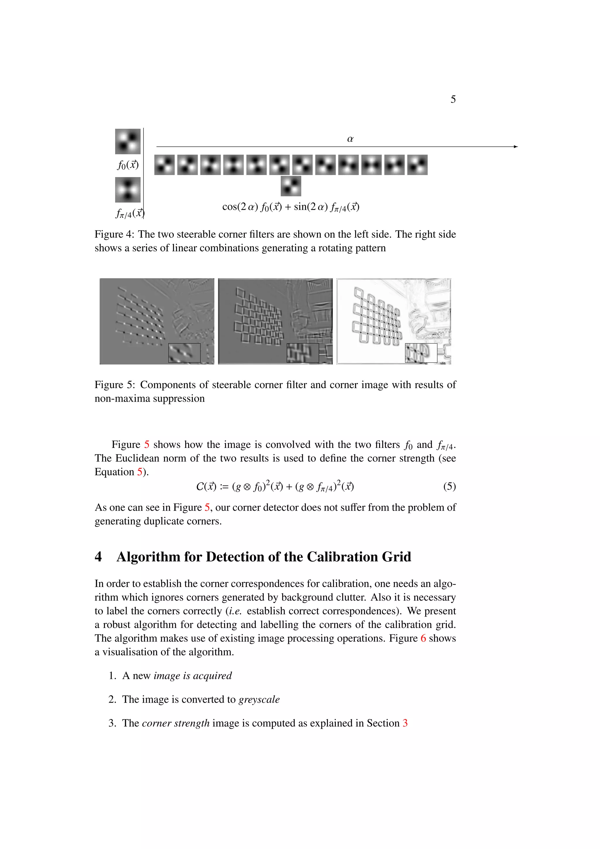
Figure 4 shows the two filters f0 and fπ/4 on the lefthand side. On the righthand
side it is shown how linear combinations of the two filters can be used to generate
a rotating pattern.
∗
sin 2 α = 2 sin α cos α and cos 2 α = cos2
α − sin2
α

5. 5
f0(x)
fπ/4(x)
α -
cos(2 α) f0(x) + sin(2 α) fπ/4(x)
Figure 4: The two steerable corner filters are shown on the left side. The right side
shows a series of linear combinations generating a rotating pattern
Figure 5: Components of steerable corner filter and corner image with results of
non-maxima suppression
Figure 5 shows how the image is convolved with the two filters f0 and fπ/4.
The Euclidean norm of the two results is used to define the corner strength (see
Equation 5).
C(x) (g ⊗ f0)2
(x) + (g ⊗ fπ/4)2
(x) (5)
As one can see in Figure 5, our corner detector does not suffer from the problem of
generating duplicate corners.
4 Algorithm for Detection of the Calibration Grid
In order to establish the corner correspondences for calibration, one needs an algo-
rithm which ignores corners generated by background clutter. Also it is necessary
to label the corners correctly (i.e. establish correct correspondences). We present
a robust algorithm for detecting and labelling the corners of the calibration grid.
The algorithm makes use of existing image processing operations. Figure 6 shows
a visualisation of the algorithm.
1. A new image is acquired
2. The image is converted to greyscale
3. The corner strength image is computed as explained in Section 3

6. 6
1. input image 2. grey scale image 3. corner strength
4. corners 5. Otsu thresholding 6. edges
7. connected components 8. component with 40
corners
9. boundary region
10. boundary corners 11. vectors 12. vectors longer than
neighbours (also see
Figure 7)
13. rounded homography
x-coordinate
14. rounded homography
y-coordinate
15. numbered corners
Figure 6: Custom algorithm for labelling the corners of a calibration grid

7. 7
0 5 10 15 20
100
150
200
corner
distancetocentre distance to centre
local maxima
Figure 7: Identifying the four extreme corners of the calibration grid by considering
the length of each vector connecting the centre with a boundary corner (also see
step 12 in Figure 6
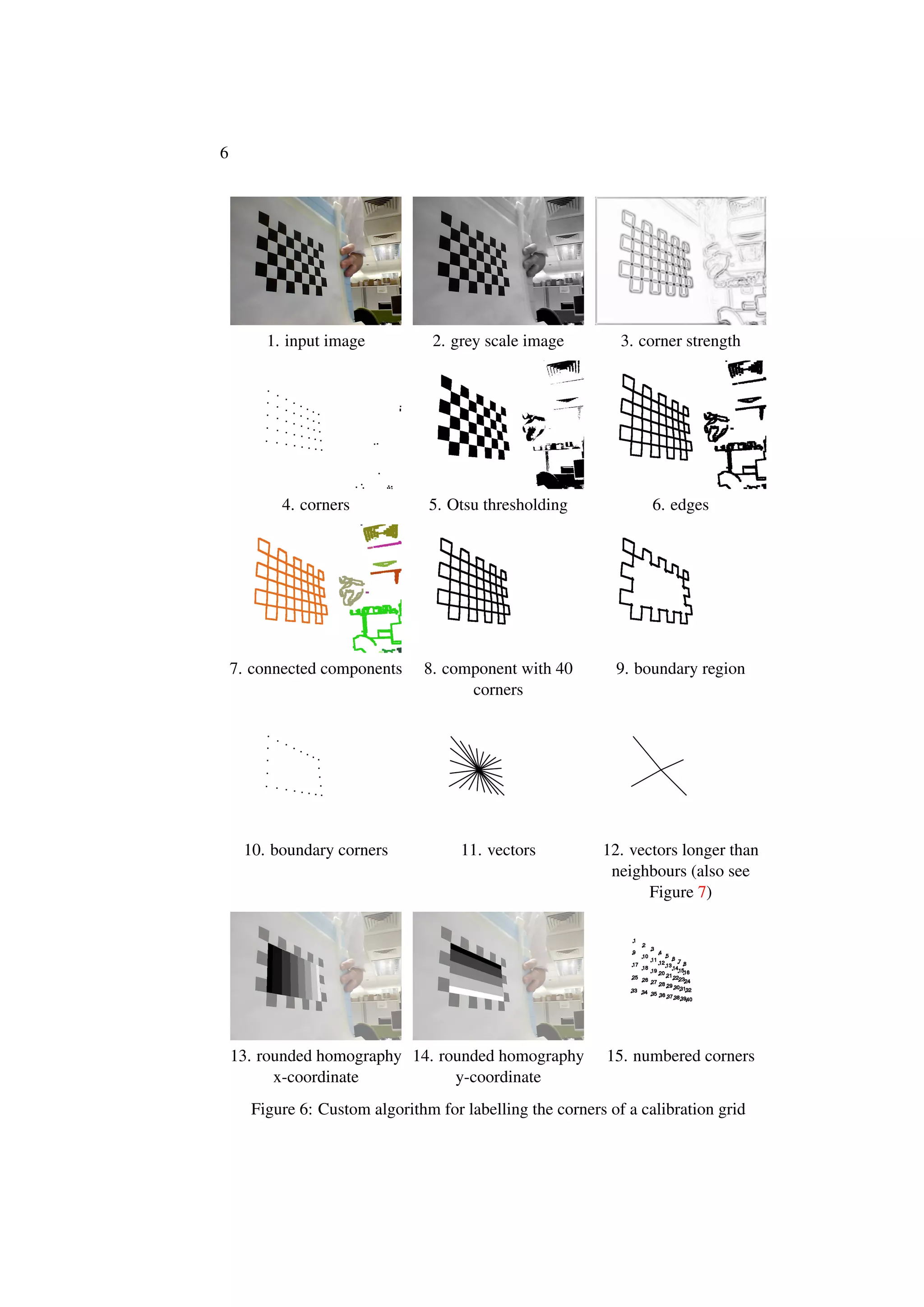
4. Non-maxima suppression for corners is used to find the local maxima in the
corner strength image (i.e. the corner locations)
5. Otsu thresholding [6] is applied to the input image. Alternatively one can
simply apply a fixed threshold
6. The edges of the thresholded image are determined using dilation and ero-
sion
7. Connected component labelling [8] is used to find connected edges
8. A weighted histogram (using the corner mask as weights) of the component
image is computed in order to find the component with 40 corners on it
9. Using connected component analysis, dilation, and logical “and” with the
grid edges, the boundary region of the grid is determined
10. Using a logical “and” with the corner mask, the boundary corners are ex-
tracted
11. The vectors connecting the centre of gravity with each boundary corner are
computed
12. The vectors are sorted by angle and vectors longer than their neighbours are
located using one-dimensional non-maxima suppression (also see Figure 7)
13. The resulting four extreme corners of the grid are used to estimate a planar
homography. The rounded x-coordinate ...
14. ... and the rounded y-coordinate of each corner can be computed now
15. The rounded homography coordinates are used to label the corners

8. 8
The algorithm needs to know the width and height in number of corners prior
to detection (here the grid is of size 8 × 5). Since it is known that there are “width
minus two” (here: 6) boundary corners between the extreme corners along the
longer side of the grid and “height minus two” (here: 3) boundary corners, it is
possible to label the corners of the calibration grid correctly except for a 180◦
ambiguity. For our purposes however it is unnecessary to resolve this ambiguity.
The algorithm is robust because it is unlikely that the background clutter causes
an edge component with exactly 40 corners. The initial homography computed
from the four extreme corners is sufficient to label all remaining corners as long as
the camera’s radial distortion is not too large.
5 Planar Homography
This section gives an outline of the method for estimating a planar homography for
a single camera picture. The method is discussed in detail in Zhengyou Zhang’s
publication [15].
The coordinate transformation from 2D coordinates on the calibration grid to
2D coordinates in the image can be formulated as a planar homography H using
homogeneous coordinates [15]. Equation 6 shows the equation for the projection
of a single point allowing for the projection error i.
∃λi ∈ R/{0} : λi




mi1
mi2
1


+


i1
i2
0




=


h11 h12 h13
h21 h22 h33
h31 h32 h33


H


mi1
mi2
1


(6)
The equations for each point can be collected in an equation system as shown
in Equation 7 by stacking the components of the unknown matrix H in a vector v
(using errors ) [15].


m11 m12 1 0 0 0 −m11 m11 −m11 m12 −m11
0 0 0 m11 m12 1 −m12 m11 −m12 m12 −m12
m21 m22 1 0 0 0 −m21 m21 −m21 m22 −m21
0 0 0 m21 m22 1 −m22 m21 −m22 m22 −m22
...
...
...
...
...
...
...
...
...


M


h11
h12
...
h33


h
=


11
12
21
22
...
n1
n2


and ||h|| = µ 0
(7)
The additional constraint ||h|| = µ 0 is introduced in order to avoid the trivial
solution. Equation 7 can be solved by computing the singular value decomposition
(SVD) so that
M = U Σ V∗
where Σ = diag(σ1, σ2, . . .)
The linear least squares solution is h = µ v9 where v9 is the right-handed singular
vector with the smallest singular value σ9 (µ is an arbitrary scale factor) [15].

9. 9
6 Calibrating the Camera
Zhengyou Zhang [15] also shows how to determine the camera intrinsic param-
eters. This section shows a simplified version of the method. The method only
determines the camera’s ratio of focal length to pixel size, i.e. we are using a per-
fect pinhole camera as a model (chip centred perfectly on optical axis, no skew, no
radial distortion). For many USB cameras this model is sufficiently accurate.
Equation 8 shows how the matrix H can be decomposed into the intrinsic ma-
trix A and extrinsic matrix R .
H =
A


f/∆s 0 0
0 f/∆s 0
0 0 1


R


r11 r12 t1
r21 r22 t2
r31 r32 t3


(8)
f/∆s is the ratio of the camera’s focal length to the physical size of a pixel on
the camera chip. The rotational part of R is an isometry [15] as formulated in
Equation 9.
R R
!
=


1 0 ∗
0 1 ∗
∗ ∗ ∗


(9)
Equation 9 also can be written using column vectors of H as shown in Equation 10
[15].
h1 A−
A−1
h2
!
= 0 and h1 A−
A−1
h1
!
= h2 A−
A−1
h2 where h1 h2 h3 H
(10)
Using Equation 8 and 10 one obtains Equation 11.
(h1,1 h1,2 + h2,1 h2,2)(∆s/ f)2
+ h3,1 h3,2
!
= 0 and
(h2
1,1 + h2
2,1 − h2
1,2 − h2
2,2)(∆s/f)2
+ h2
3,1 − h2
3,2
!
= 0
(11)
In general this is a overdetermined equation system which does not have a solution.
Therefore the least squares algorithm is used in order to find a value for (∆s/f)2
which minimises the left-hand terms shown in Equation 11. Furthermore the least
squares estimation is performed for a set of frames in order to get a more robust
estimate for f/∆s. That is, every frame (with successfully recognised calibration
grid) contributes two additional equations for the least squares fit.
7 Results
We have implemented the camera calibration using the Ruby† programming lan-
guage and the HornetsEye library. Figure 8 shows the result of applying the algo-
rithm to a test video. The figure shows the individual estimate for each frame and a
†
http://www.ruby-lang.org/

10. 10
0 100 200 300 400 500 600 700 800
0
500
1,000
1,500
2,000
camera frame
f/∆s
frames shown in Figure 9
single frame estimate
cumulative estimate
Figure 8: Estimate for f/∆s for real test video
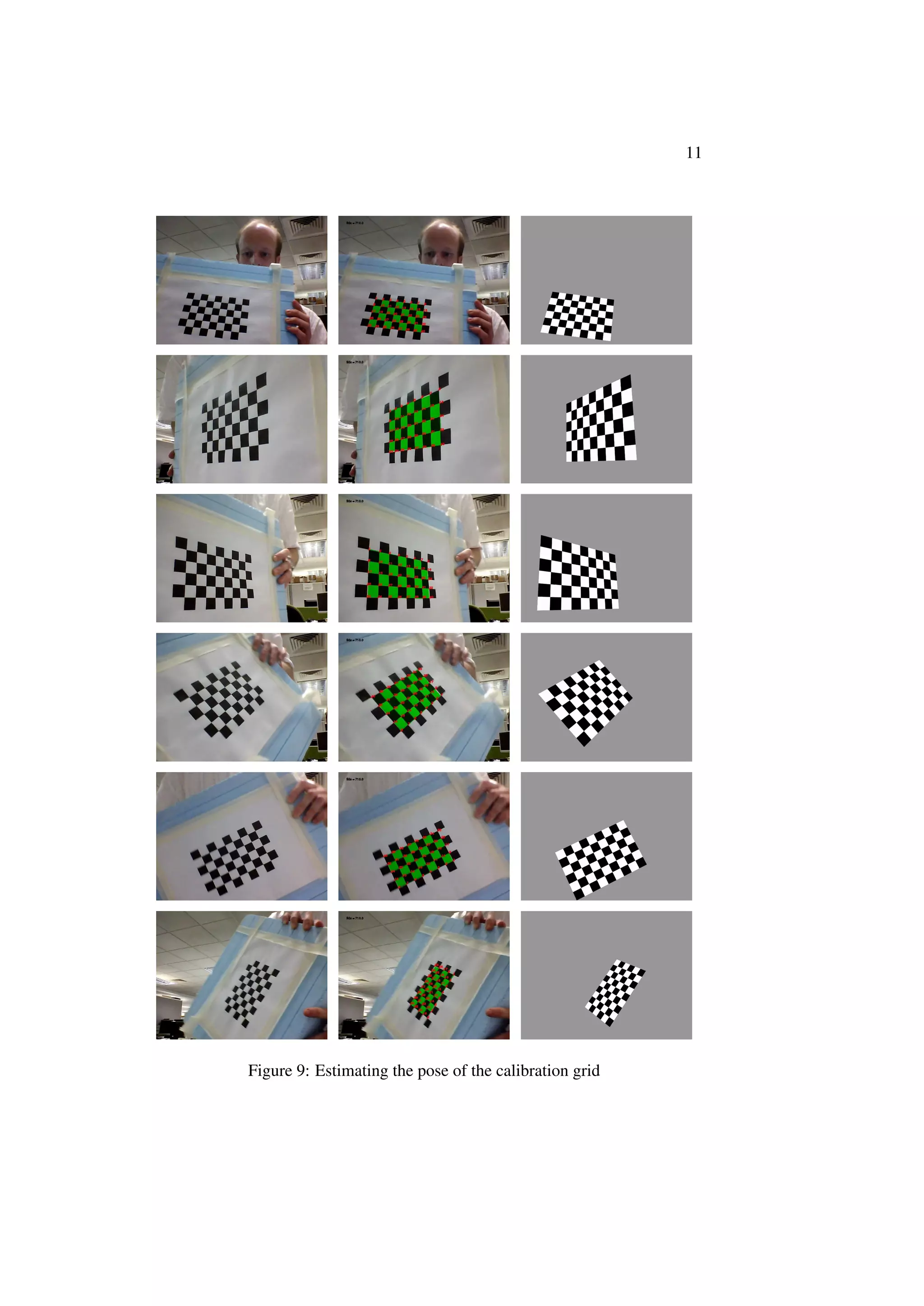
cumulative estimate which improves over time. A few individual frames are shown
in Figure 9. One can see that the bad estimate occur when the calibration grid is
almost parallel to the projection plane of the camera. Also the individual estimates
are biased which might be caused by motion blur, bending of the calibration sur-
face, and by the device not being an ideal pinhole camera.
In order to validate the calibration method, the sequence of poses from the real
video was used to render an artificial video assuming a perfect pinhole camera. The
result is shown in Figure 10. One can see that the bias is negligible. The bias could
be reduced by using sub-pixel refinement of the corner locations (e.g. as shown in
[3]). Furthermore in order to achieve the closed solution for the planar homography
(see Section 5) it was necessary to use errors which only have approximately equal
variance. However the final estimate for f/∆s already has an error of less than 1 .
8 Conclusion
We have presented a novel method for localising a chequer board for camera cali-
bration. The method is robust and it does not require user interaction. A steerable
filter pair was used to detect the corners of the calibration grid. The algorithm
for isolating and labelling the corners of the calibration grid is based on standard
image processing operations and thus can be implemented easily.
A simplified version of Zhengyou Zhang’s calibration method [15] using a pin-
hole camera model was used. The algorithm works well on real images taken with
a USB webcam. The method was validated on an artificial video to show that the
bias of the algorithm is negligible and that the algorithm converges on the correct
solution.
The algorithm was implemented using the Ruby programming language and
the HornetsEye‡ machine vision library. The implementation is available online§.
Possible future work is to develop steerable filters which can be steered in both
location as well as rotation in order to detect edges with sub-pixel accuracy.
‡
http://www.wedesoft.demon.co.uk/hornetseye-api/
§
http://www.wedesoft.demon.co.uk/hornetseye-api/calibration.rb

11. 11
Figure 9: Estimating the pose of the calibration grid

12. 12
0 100 200 300 400 500 600 700 800
0
500
1,000
1,500
2,000
camera frame
f/∆s
single frame estimate
cumulative estimate
Figure 10: Estimate for f/∆s for artificial video
References
[1] D. H. Ballard and C. M. Brown. Computer Vision. Prentice Hall, 1982. 2
[2] J.-Y. Bouguet. Camera calibration toolbox for Matlab, 2010. 3
[3] D. Chen and G. Zhang. A new sub-pixel detector for x-corners in camera
calibration targets. In 13th International Conference in Central Europe on
Computer Graphics, Visualization and Computer Vision. Citeseer, 2005. 10
[4] C. G. Harris and M. Stephens. A combined corner and edge detector. Pro-
ceedings 4th Alvey Vision Conference, pages 147–151, 1988. 3
[5] G. Heidemann. The principal components of natural images revisited. Pattern
Analysis and Machine Intelligence, IEEE Transactions on, 28(5):822–826,
2006. 4
[6] N. Otsu. A threshold selection method from gray-level histograms. Systems,
Man and Cybernetics, IEEE Transactions on, 9(1):62–66, Jan. 1979. 7
[7] T. Pachidis, J. Lygouras, and V. Petridis. A novel corner detection algorithm
for camera calibration and calibration facilities. Recent Advances in Circuits,
Systems and Signal Processing, pages 338–343, 2002. 3
[8] J.-M. Park, C. G. Looney, and H.-C. Chen. Fast connected component label-
ing algorithm using a divide and conquer technique. In 15th International
Conference on Computers and their Applications, Proceedings of CATA-
2000, pages 373–6, Mar. 2000. 7
[9] M. Pollefeys, L. V. Gool, M. Vergauwen, F. Verbiest, K. Cornelis, J. Tops, and
R. Koch. Visual modeling with a hand-held camera. International Journal of
Computer Vision, 59(3):207–32, 2004. 1
[10] L. Robert. Camera calibration without feature extraction. Computer Vision
and Image Understanding, 63(2):314–325, 1996. 3

13. 13
[11] J. Shi and C. Tomasi. Good features to track. In Proceedings of the 1994 IEEE
Computer Society Conference on Computer Vision and Pattern Recognition,
pages 593–600, June 1994. 3
[12] R. Tsai. A versatile camera calibration technique for high-accuracy 3d ma-
chine vision metrology using off-the-shelf tv cameras and lenses. Robotics
and Automation, IEEE Journal of, 3(4):323–344, 1987. 2
[13] Z. Wang, Z. Wang, and Y. Wu. Recognition of corners of planar checkboard
calibration pattern image. In Control and Decision Conference (CCDC), 2010
Chinese, pages 3224–3228, May 2010. 3
[14] J. Wedekind, B. P. Amavasai, and K. Dutton. Steerable filters generated with
the hypercomplex dual-tree wavelet transform. In 2007 IEEE International
Conference on Signal Processing and Communications, pages 1291–4. 4
[15] Z. Zhang. A flexible new technique for camera calibration. Pattern Analysis
and Machine Intelligence, IEEE Transactions on, 22(11):1330–1334, 2000.
2, 3, 8, 9, 10