Download to read offline
![Lossy Compression
• Based on spatial redundancy
• Measure of spatial redundancy: 2D covariance
• CovX(i,j)= σ2
e-α√(i*i+j*j)
• Vertical correlation ρ1=
• Horizontal correlation ρ2=
• For images we assume equal correlations
• Typically e-α
= ρ1= ρ2= 0.95
• Measure of loss (or distortion):
• MSE between encoded and decoded image
E[X(i,j)X(i-1,j)]
E[X2
(i,j)]
E[X(i,j)X(i,j-1)]
E[X2
(i,j)]](https://image.slidesharecdn.com/mmclass4-140513063953-phpapp02/85/Mmclass4-1-320.jpg)
![Lossy Compression
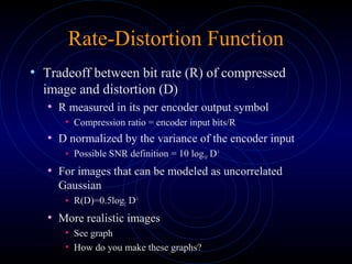
• Based on spatial redundancy
• Measure of spatial redundancy: 2D covariance
• CovX(i,j)= σ2
e-α√(i*i+j*j)
• Vertical correlation ρ1=
• Horizontal correlation ρ2=
• For images we assume equal correlations
• Typically e-α
= ρ1= ρ2= 0.95
• Measure of loss (or distortion):
• MSE between encoded and decoded image
E[X(i,j)X(i-1,j)]
E[X2
(i,j)]
E[X(i,j)X(i,j-1)]
E[X2
(i,j)]](https://image.slidesharecdn.com/mmclass4-140513063953-phpapp02/75/Mmclass4-1-2048.jpg)
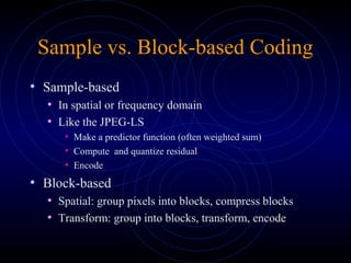
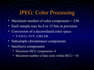
![JPEG: Quantization Tables
• 8 X 8 quantization table for each image
component
• Q(i,j): quantization step for corresponding DCT
element
• 1 ≤ Q(i,j) ≤ 255
• Psycho-visual experiments
• Bit-rate control
• Total number of block = B
• yk[i,j] : (i,j) output of k-th block
∑∑= =
=
8
1
8
164
1
i i
ij rb target av. bit-rate
bits per DCT coeff
64
,
])],[([
]),[(
2log
2
1
∏
+=
ji
jiyVar
jiyVar
ij rb ijb
jiQ
2
2046
],[ = for 8-bit images](https://image.slidesharecdn.com/mmclass4-140513063953-phpapp02/85/Mmclass4-8-320.jpg)
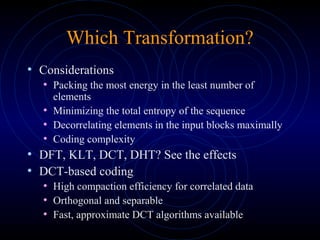
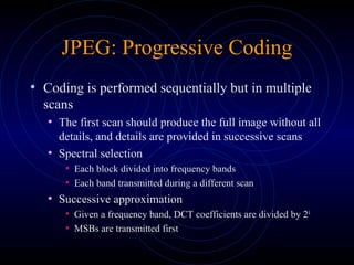
![JPEG: Entropy Coding
• Baseline processing
• Total of 4 code tables allowed
• Different code tables for luminance and chrominance
• DC coefficients
• DC differentials are computed and have the range [-2047, 2047]
• The range is divided into 12 size categories
• Category i needs i bits to represent the value
• DC residuals are represented as [size, amplitude] pairs
• Size is Huffman encoded](https://image.slidesharecdn.com/mmclass4-140513063953-phpapp02/85/Mmclass4-9-320.jpg)
![JPEG: Entropy Coding
• AC coefficients
• Take value in the range [-1023, 1023]
• 10 size categories
• Only non-zero coefficients need to be encoded
• Processed in zig-zag order
• More efficient run-length encoding of AC coefficients
• Represented as (run/size, amplitude)
• If run > 15, possibly several (15/0) symbols are used](https://image.slidesharecdn.com/mmclass4-140513063953-phpapp02/85/Mmclass4-10-320.jpg)
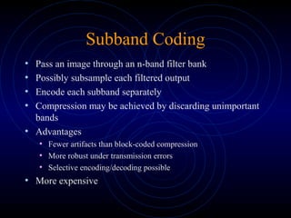
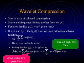

This document discusses different techniques for lossy image compression including JPEG. It describes lossy compression being based on spatial redundancy and using a covariance measure. It then discusses rate-distortion functions and how they relate compression ratio and distortion. It provides details on sample-based and block-based coding approaches as well as considerations for different transformations like DCT. The document outlines the JPEG encoding process including color processing, quantization tables, and entropy coding methods. It also discusses progressive coding and subband coding techniques.