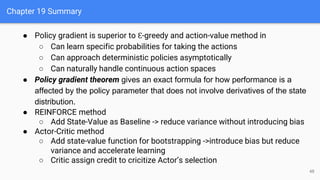
The document provides an extensive overview of policy gradient methods in reinforcement learning, detailing various algorithms such as REINFORCE, actor-critic methods, and deterministic policy gradient. It emphasizes the advantages of policy gradients over value-based methods, particularly in their ability to handle continuous action spaces and specific action probabilities. Key topics include the policy gradient theorem, exploration strategies, and the integration of state-value functions to improve learning efficiency and reduce variance.

1. Policy Gradient (Part 1)
Reinforcement Learning : An Introduction 2e, 2018.July
Bean https://www.facebook.com/littleqoo
1

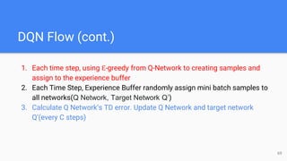
2. Agenda
Reinforcement Learning：An Introduction
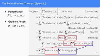
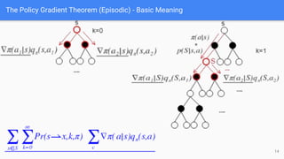
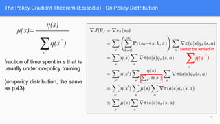
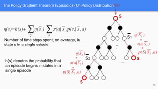
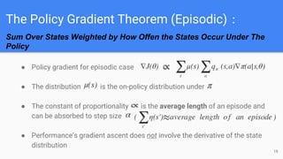
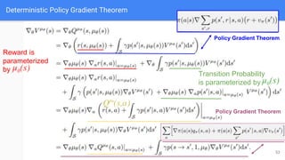
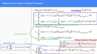
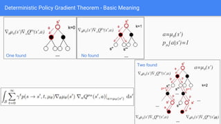
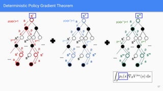
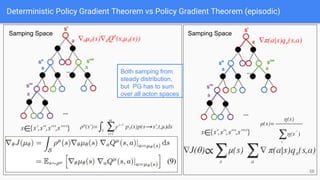
● Policy Gradinet Theorem
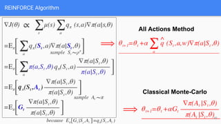
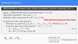
● REINFORCE: Monte -Carlo Policy Gradient
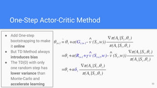
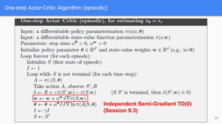
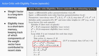
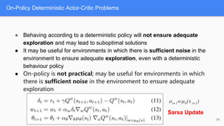
● One-Step Actor Critic
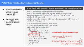
● Actor Critic with Eligibility Trace (Eposodic and Continuing Case)
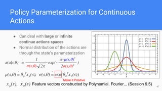
● Policy Parameterization for Continuous Actions
DeepMind (Richard Sutton、David Silver)
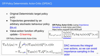
● Determinstic Policy Gradient (DPG(2014)、DDPG(2016)、MADDPG(2018)[part 2])
● Distributed Proximal Policy Optimization(DPPO 2017.07) [part 2]
OpenAI (Pieter Abbeel、John Schulman)
● Trust Region Policy Gradient (TRPO(2016)) [part 2]
● Proximal Policy Optimization (PPO(2017.07)) [part 2]
2

3. Reinforcement Learning Classification
● Value-Based
○ Learned Value Function
○ Implicit Policy
(usually Ɛ-greedy)
● Policy-Based
○ No Value Function
○ Explicit Policy
Parameterization
● Mixed(Actor-Critic)
○ Learned Value Function
○ Policy Parameterization
3

4. Policy Gradient Method
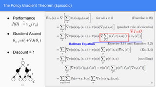
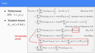
Goal：
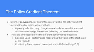
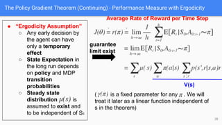
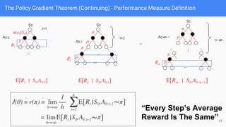
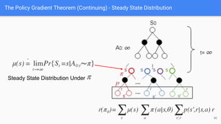
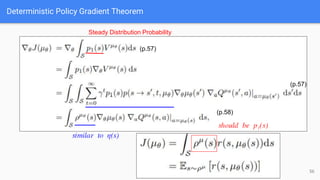
Performance Messure：
Optimization：Gradient Ascent
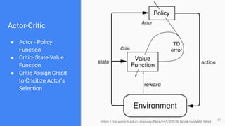
[Actor-Critic Method]：Learn approximation to both policy and value
function
4

5. Policy Approximation (Discrete Actions)
● Ensure exploration we generally require that the policy never becomes
deterministic
● The most common parameterization for discrete action spaces - Softmax
in action preferences
○ discrete action space can not too large
● Action preferences can be
parameterization arbitrarily(linear, ANN...)
5

6. Advantage of Policy Approximation
1. Can approach to a deterministic policy (Ɛ-
greedy always has Ɛ probability of selecting
a random action),ex: Temperature parameter
(T -> 0) of soft-max
○ In practice, it is difficult to choose reduction
schedule or initial value of T
2. Enables the selection of actions with
arbitrary probabilities
○ Bluffing in poker, Action-Value methods have no
natural way
6

7. https://en.wikipedia.org/wiki/Softmax_function (Temperature parameters)
3. May be simpler function to approximate depending on the complexity
of
policies and action-value functions
4. A good way of injecting prior knowledge about the desired form of the
policy into the reinforcement learning system (often the most important
reason)
7

8. Short Corridor With Switched Actions
● All the states appear
identical under the function
approximation
● A method can do
significantly better if it can
learn a specific probability
with which to select right
● The best probability is
about 0.59
8

9. The Policy Gradient Theorem (Episodic)
https://papers.nips.cc/paper/1713-policy-gradient-methods-for-reinforcement-
learning-with-function-approximation.pdf
NIPS 2000 Policy Gradient Methods for Reinforcement Learning with Function
Approximation (Richard S. Sutton)
9

10. The Policy Gradient Theorem
● Stronger convergence of guarantees are available for policy-gradient
method than for action-value methods
○ Ɛ-greedy selection may change dramatically for an arbitrary small
action value change that results in having the maximal value
● There are two cases define the different performance messures
○ Episodic Case - performance measure as the value of the start state
of the episode
○ Continuing Case - no end even start state (Refer to Chap10.3)
10

11. The Policy Gradient Theorem (Episodic)
● Performance
● Gradient Ascent
● Discount = 1
Bellman Equation
11

12. Cont.
● Performance
● Gradient Ascent
recurisively
unroll
12

13. The Policy Gradient Theorem (Episodic)
● Performance
● Gradient Ascent
13

14. The Policy Gradient Theorem (Episodic) - Basic Meaning
14

15. The Policy Gradient Theorem (Episodic) - On Policy Distribution
fraction of time spent in s that is
usually under on-policy training
(on-policy distribution, the same
as p.43)
15
better be writed in

16. The Policy Gradient Theorem (Episodic) - On Policy Distribution
Number of time steps spent, on average, in
state s in a single episoid
h(s) denotes the probability that
an episode begins in states in a
single episode
16

17. The Policy Gradient Theorem (Episodic) - Concept
17
Ratio of s that
appear in the
state-action tree
Gathering gradients over all action
spaces of every state

18. The Policy Gradient Theorem (Episodic)：
Sum Over States Weighted by How Offen the States Occur Under The
Policy
● Policy gradient for episodic case
● The distribution is the on-policy distribution under
● The constant of proportionality is the average length of an episode and
can be absorbed to step size
● Performance’s gradient ascent does not involve the derivative of the state
distribution
18

19. REINFORCE : Monte-Carlo Policy Gradient
Classical Policy Gradient
19

20. REINFORCE Algorithm
All Actions Method
Classical Monte-Carlo
20

21. REINFORCE Meaning
● The update increases the
parameter vector in this
direction proportional
to the return
● inversely proportional to the
action probability (make sense
because otherwise actions that
are selected frequently are at an
advantage)
Action is a summation. If using
samping by action probability, we
have to average gradient by sampling
number
21

22. REINFORCE Algorithm
Wait Until One Episode Generated
22

23. REINFORCE on the short-corridor gridworld
short-corridor gridworld
● With a good step
size, the total
reward per episode
approaches the
optimal value of the
start state
23

24. REINFORCE Defect & Solution
● Slow Converage
● High Variance From Reward
● Hard To Choose Learning Rate
24

25. REINFORCE with Baseline (episodic)
● Expected value of the update
unchanged(unbiased), but it
can have a large effect on its
variance
● Baseline can be any function,
evan a random variable
● For MDPs, the baseline should
vary with state, one natural
choice is state value function
○ some states all actions
have high values => a high
baseline
○ in others, => a low baseline
Treat State-Value Function as
a Independent Value-function
Approximation!
25

26. REINFORCE with Baseline (episodic)
can be learned by any methods
of previous chapters independently.
We use the same Monte-Carlo
here.(Section 9.3 Gradient Monte-Carlo)
26

27. Short-Corridor GridWorld
● Learn much
faster
● Policy
parameter is
much less clear
to set
● State-Value
function
paramenter
(Section 9.6)
27

28. Defects
● Learn Slowly (product estimates of high variance)
● Incovenient to implement online or continuing problems
28

29. Actor-Critic Methods
Combine Policy Function with Value Function
29

30. One-Step Actor-Critic Method
● Add One-step
bootstrapping to make
it online
● But TD Method always
introduces bias
● The TD(0) with only
one random step has
lower variance than
Monte-Carlo and
accelerate learning 30

31. Actor-Critic
● Actor - Policy
Function
● Critic- State-Value
Function
● Critic Assign Credit
to Cricitize Actor’s
Selection
31
https://cs.wmich.edu/~trenary/files/cs5300/RLBook/node66.html

32. One-step Actor-Critic Algorithm (episodic)
Independent Semi-Gradient TD(0)
(Session 9.3)
32

33. Actor-Critic with Eligiblity Traces (episodic)
● Weight Vector
is a long-term
memory
● Eligibility trace
is a short-term
memory,
keeping track
of which
components of
the weight
vector have
contributed to
recent state
33

34. Review of Eligibility Traces - Forward View (Optional)
34

35. Review of Eligibility Traces - Forward View (Optional)
TD(0)
TD(1)
TD(2)
35
My Eligibility Trace Indution Link https://cacoo.com/diagrams/gof2aiV3fCXFGJXF

36. Review of Eligibility Traces - Backward View vs Momentum (Optional)
Example：
Eligibility Traces Gradient Momentum
similiar
Accumulate Decayed Gradient
36

37. The Policy Gradient Theorem (Continuing)
37

38. The Policy Gradient Theorem (Continuing) - Performance Measure with Ergodicity
● “Ergodicity Assumption”
○ Any early decision by
the agent can have
only a temporary
effect
○ State Expectation in
the long run depends
on policy and MDP
transition
probabilities
○ Steady state
distribution is
assumed to exist and
to be independent of S0
guarantee
limit exist
Average Rate of Reward per Time Step
38
( is a fixed parameter for any . We will
treat it later as a linear function independent of
s in the theorem)
V(s)

39. The Policy Gradient Theorem (Continuing) - Performance Measure Definition
“Every Step’s Average
Reward Is The Same”39

40. The Policy Gradient Theorem (Continuing) - Steady State Distribution
Steady State Distribution Under
40

41. Replace Discount with Average Reward for Continuing Problem(Session 10.3, 10.4)
● Continuing problem with discounted setting is useful in tabular case, but
questionable for function approximation case
● In Continuing problem, performance measure with discounted setting is
proportional to the average reward setting (They has almost the same
effect )(session 10.4)
● Discounted setting is problematic with function approximation
○ with function approximation we have lost the policy improvement
theorem (session 4.3) important in Policy Iteration Method
41

42. Proof The Policy Gradient Theorem (Continuing) 1/2
Gradient Definition
Parameterization of policy
by replacing discount with
average reward setting 42

43. Proof The Policy Gradient Theorem (Continuing) 2/2
● Introduce
steady state
distribution
and its
property
steady state distribution property
43
By Definistion, it’s independent of s
Trick

44. Steady State Distribution Property
44

45. Policy Gradient Theorem (Continuing) Final Concept
45

46. Actor-Critic with Eligibility Traces (continuing)
● Replace Discount
with average
reward
● Traing with
Semi-Gradient
TD(0)
Independent Semi-Gradient TD(0)
=1
46

47. Policy Parameterization for Continuous
Actions
● Can deal with large or infinite
continue actions spaces
● Normal distribution of the actions are
through the state’s parameterization
Feature vectors constructed by Polynomial, Fourier... (Session 9.5) 47
Make it Positive

48. Chapter 19 Summary
● Policy gradient is superior to Ɛ-greedy and action-value method in
○ Can learn specific probabilities for taking the actions
○ Can approach deterministic policies asymptotically
○ Can naturally handle continuous action spaces
● Policy gradient theorem gives an exact formula for how performance is a
affected by the policy parameter that does not involve derivatives of the state
distribution.
● REINFORCE method
○ Add State-Value as Baseline -> reduce variance without introducing bias
● Actor-Critic method
○ Add state-value function for bootstrapping ->introduce bias but reduce
variance and accelerate learning
○ Critic assign credit to cricitize Actor’s selection
48

49. Deterministic Policy Gradient
(DPG)
http://proceedings.mlr.press/v32/silver14.pdf
http://proceedings.mlr.press/v32/silver14-supp.pdf
ICML 2014 Deterministic Policy Gradient Algorithms (David Silver)
49

50. Comparison with Stochastic Policy Gradient
Advantage
● No action space sampling, more efficient (usually 10x faster)
● Can deal with large action space more efficiently
Weekness
● Less Exploration
50

51. Deterministic Policy Gradient Theorem - Performance Measure
● Deterministic Policy
Performance Messure
51
● Policy Gradient (Continuing)
Performance Messure
(Paper Not Distinguishing from
Episodic to Continuing Case)
Similar to
V(s)
V(s)

52. Deterministic Policy Gradient Theorem - Gradient
52
● Policy Gradient
(Continuing)
● Deterministic Policy
Gradient

53. Deterministic Policy Gradient Theorem
Policy Gradient Theorem
Transition Probability
is parameterized by
Policy Gradient Theorem
53
Reward is
parameterized
by

54. Deterministic Policy Gradient Theorem
Policy Gradient Theorem
Unrolling
54
Combination
coverage cues

55. Deterministic Policy Gradient Theorem - Basic Meaning
55
No foundOne found
Two found
p=1p=1

56. Deterministic Policy Gradient Theorem
56
Steady Distribution Probability
(p.57)
(p.57)
(p.58)

57. Deterministic Policy Gradient Theorem
57
p=1 p=1 p=1 p=1 p=1 p=1
p(a|s’)=1 p(a|s’’)=1 p(a|s’’’)=1

58. Deterministic Policy Gradient Theorem vs Policy Gradient Theorem (episodic)
58
Both samping from
steady distribution,
but PG has to sum
over all acton spaces
Samping Space Samping Space

59. On-Policy Deterministic Actor-Critic Problems
59
● Behaving according to a deterministic policy will not ensure adequate
exploration and may lead to suboptimal solutions
● It may be useful for environments in which there is sufficient noise in the
environment to ensure adequate exploration, even with a deterministic
behaviour policy
● On-policy is not practical; may be useful for environments in which
there is sufficient noise in the environment to ensure adequate
exploration
Sarsa Update

60. Off-Policy Deterministic Actor-Critic (OPDAC)
● Original Deterministic target policy
µθ(s)
● Trajectories generated by an
arbitrary stochastic behaviour policy
β(s,a)
● Value-action function off-policy
update - Q learning
60
Off Policy Actor-Critic (using Importance
Sampling in both Actor and Critic)
https://arxiv.org/pdf/1205.4839.pdf
Off Policy Deterministic Actor-Critic
DAC removes the integral
over actions, so we can avoid
importance sampling in the
actor

61. Compatible Function Approximation
61
● For any deterministic policy (s), there always exists a compatible function
approximator of

62. Off-Policy Deterministic Actor-Critic (OPDAC)
62
Actor
Critic

63. Experiments Designs
63
1. Continus Bandit, with fixed width Gaussian
behaviro policy
2. Mountain Car, with fixed width
Gaussian behavior policy
3. Octopus Arm with 6 segments
a. Sigmoidal multi-layer perceptron (8 hidden units and sigmoidal output units) to represent
the policy (s)
b. A(s) function approximator (session 4.3)
c. V(s) multi-layer perceptron (40 hidden units and linear output units).

64. Experiment Results
64
In practice, the DAC significantly outperformed its stochastic counterpart by several
orders of magnitude in a bandit with 50 continuous action dimensions, and solved a
challenging reinforcement learning problem with 20 continuous action dimensions
and 50 state dimensions.

65. Deep Deterministic Policy
Gradient (DDPG)
https://arxiv.org/pdf/1509.02971.pdf
ICLR 2016 Continuous Control With Deep Reinforcement Learning (DeepMind)
65

66. Q-Learning Limitation
66
http://doremi2016.logdown.com/posts/2017/01/25/convolutional-neural-networks-cnn my cnn architecture
http://www.davidqiu.com:8888/research/nature14236.pdf Human-level control through deep reinforcement learning
Tabular Q-learning Limitations
● Very limited states/actions
● Can’t generalize to unobserved states
Q-learning with function approximation(neural net) can solve limits
above but still unstable or diverge
● The correlations present in the sequence of observations
● Small updates to Q function may significantly change the
policy(policy may oscillate)
● Scale of rewards vary greatly from game to game
○ lead to largely unstable gradient caculation

67. Deep Q-Learning
67http://www.davidqiu.com:8888/research/nature14236.pdf Human-level control through deep reinforcement learning
1. Experimence Replay
○ Break samples’
correlations
○ Off-policy learn for
all past policies
2. Independent Target Q-
network and update
weight from Q-network
every C steps
○ Avoid oscillations
○ Break correlations
with Q-network
3. Clip rewards to limit the
scale of TD error
○ Robust Gradinet
behavior policy Ɛ-greedy
experience replay buffer
Freeze and update Target Q network
train
minibach
size samples

68. 68
modify from https://blog.csdn.net/u013236946/article/details/72871858
DQN Flow

69. DQN Flow (cont.)
69
1. Each time step, using Ɛ-greedy from Q-Network to creating samples and
assign to the experience buffer
2. Each Time Step, Experience Buffer randomly assign mini batch samples to
all networks(Q Network, Target Network Q’)
3. Calculate Q Network’s TD error. Update Q Network and target network
Q’(every C steps)

70. DQN Disadvantage
● Many tasks of interest, most notably physical control tasks, have
continuous (real valued) and high dimensional action spaces
● With high-dimensional observation spaces, it can only handle discrete and
low-dimensional action spaces (requires an iterative optimization process
at every step to find the argmax)
● Simple Approach for DQN to deal with continus domain is simply
discretizing，but many limitation：the number of actions increases
exponentially with the number of degrees of freedom，ex：a 7 degree of
freedom system (as in the human arm) with the coarsest discretization a ∈
{−k, 0, k} for each joint. 3^7 = 2187 action dimensionality
70
https://arxiv.org/pdf/1509.02971.pdf CONTINUOUS CONTROL WITH DEEP REINFORCEMENT LEARNING

71. DDPG Contributions (DQN+DPG)
71
● Can learn policies “end-to-end”：directly from raw pixel inputs (DQN)
● Can learn policies from high-dimentional continus action space (DPG)
● From above, we can learn policies in large state and action space online

72. 72
DDPG Algo
● Experience
Replay
● Independent
Target
networks
● Batch
Normalization
of Minibatch
● Temporal
Correlated
Exploration
temporal correlated random policy
experience replay buffer
mini batch
Train Actor
mini batch
Train Critic
weighted blending between Q and Target Q’ network
weighted blending between Actor μ and Target Actor μ’network

73. DDPG Flow
73

74. DDPG Flow (cont.)
74
1. Each time step, using temporally correlated policy to create a sample and
assign it to experience replay buffer
2. Each time step, experience buffer assign mini batch samples to all
networks(Actor μ, Actor Target μ’, Q Network, Q' Target Network)
3. Calculate Q Network’s TD error. Update Q Network and Q' target network
Calculate Actor’s gradient. Update μ and target μ’

75. DDPG Challenges and Solutions
75
● Replay Buffer is used to break up sequeitial samples (like DQN)
● Target Networks is used for stable learning, but use “soft” update
○
○ Target networks slowly change, but greatly improve the stability of
learning
● Using Batch Normalization to normalize each dimension across the
minibatch samples (in low dimensional feature space, observation may
have different physical values, like position and velocity)
● Use Ornstein-Uhlenbeck process to generate temporally correlated
exploration efficiency with inertia

76. Applications
76