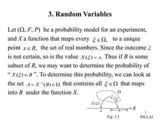
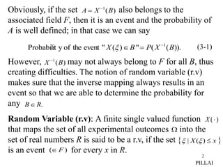
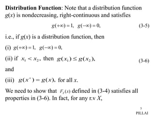
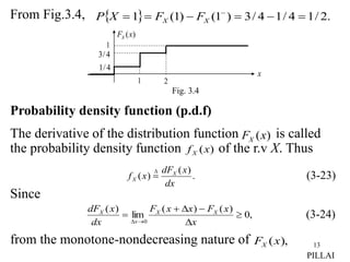
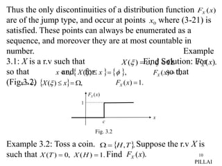
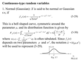
1. A random variable (X) is a function that maps outcomes of a probability experiment to real numbers. The probability distribution function (FX(x)) gives the probability that X takes on a value less than or equal to x. 2. FX(x) satisfies properties of a distribution function - it is nondecreasing, right-continuous, and its limit as x approaches positive/negative infinity is 0/1. 3. A random variable can be either continuous or discrete. FX(x) is continuous if it is continuous for all x, and discrete if it has jump discontinuities at countable points.

1. 1
3. Random Variables
Let (, F, P) be a probability model for an experiment,
and X a function that maps every to a unique
point the set of real numbers. Since the outcome
is not certain, so is the value Thus if B is some
subset of R, we may want to determine the probability of
“ ”. To determine this probability, we can look at
the set that contains all that maps
into B under the function X.
,



,
R
x 
.
)
( x
X 

B
X 
)
(


 
)
(
1
B
X
A 




R
)
(
X
x
A
B
Fig. 3.1 PILLAI

2. 2
Obviously, if the set also belongs to the
associated field F, then it is an event and the probability of
A is well defined; in that case we can say
However, may not always belong to F for all B, thus
creating difficulties. The notion of random variable (r.v)
makes sure that the inverse mapping always results in an
event so that we are able to determine the probability for
any
Random Variable (r.v): A finite single valued function
that maps the set of all experimental outcomes into the
set of real numbers R is said to be a r.v, if the set
is an event for every x in R.
)
(
1
B
X
A 

)).
(
(
"
)
(
"
event
the
of
y
Probabilit 1
B
X
P
B
X 


 (3-1)
)
(
1
B
X 
.
R
B 
)
( 
X

 
)
(
| x
X 


)
( F

PILLAI

3. 3
Alternatively X is said to be a r.v, if where B
represents semi-definite intervals of the form
and all other sets that can be constructed from these sets by
performing the set operations of union, intersection and
negation any number of times. The Borel collection B of
such subsets of R is the smallest -field of subsets of R that
includes all semi-infinite intervals of the above form. Thus
if X is a r.v, then
is an event for every x. What about
Are they also events ? In fact with since
and are events, is an event and
hence is also an event.
}
{ a
x 


a
b 
   ?
, a
X
b
X
a 


 
b
X 
    }
{ b
X
a
b
X
a
X 





   
a
X
a
X
c



   
)
(
| x
X
x
X 




F
B
X 

)
(
1
}
{ a
X 
(3-2)
PILLAI

4. 4
Thus, is an event for every n.
Consequently
is also an event. All events have well defined probability.
Thus the probability of the event must
depend on x. Denote
The role of the subscript X in (3-4) is only to identify the
actual r.v. is said to the Probability Distribution
Function (PDF) associated with the r.v X.









1
a
X
n
a














1
}
{
1
n
a
X
a
X
n
a
 
)
(
| x
X 


  .
0
)
(
)
(
| 

 x
F
x
X
P X

 (3-4)
)
(x
FX
(3-3)
PILLAI

5. 5
Distribution Function: Note that a distribution function
g(x) is nondecreasing, right-continuous and satisfies
i.e., if g(x) is a distribution function, then
(i)
(ii) if then
and
(iii) for all x.
We need to show that defined in (3-4) satisfies all
properties in (3-6). In fact, for any r.v X,
,
0
)
(
,
1
)
( 


 g
g
,
0
)
(
,
1
)
( 


 g
g
,
2
1 x
x  ),
(
)
( 2
1 x
g
x
g 
),
(
)
( x
g
x
g 

(3-6)
)
(x
FX
(3-5)
PILLAI

6. 6
  1
)
(
)
(
|
)
( 





 P
X
P
FX 

  .
0
)
(
)
(
|
)
( 




 

 P
X
P
FX
(i)
and
(ii) If then the subset
Consequently the event
since implies As a result
implying that the probability distribution function is
nonnegative and monotone nondecreasing.
(iii) Let and consider the event
since
,
2
1 x
x  ).
,
(
)
,
( 2
1 x
x 


   ,
)
(
|
)
(
| 2
1 x
X
x
X 

 



1
)
( x
X 
 .
)
( 2
x
X 

    ),
(
)
(
)
(
)
( 2
2
1
1 x
F
x
X
P
x
X
P
x
F X
X 



 
 (3-9)
 
(3-7)
(3-8)
,
1
2
1 x
x
x
x
x n
n 



  
 .
)
(
| k
k x
X
x
A 

 
 (3-10)
     ,
)
(
)
(
)
( k
k x
X
x
X
x
X
x 




 

 (3-11)
PILLAI

7. 7
using mutually exclusive property of events we get
But and hence
Thus
But the right limit of x, and hence
i.e., is right-continuous, justifying all properties of a
distribution function.
  ).
(
)
(
)
(
)
( x
F
x
F
x
X
x
P
A
P X
k
X
k
k 



  (3-12)
,
1
1 
 
 
 k
k
k A
A
A
.
0
)
(
lim
hence
and
lim
1









k
k
k
k
k
k
A
P
A
A 
 (3-13)
.
0
)
(
)
(
lim
)
(
lim 






x
F
x
F
A
P X
k
X
k
k
k
),
(
)
( x
F
x
F X
X 

)
(x
FX
(3-14)
,
lim 


 x
xk
k
PILLAI

8. 8
Additional Properties of a PDF
(iv) If for some then
This follows, since implies
is the null set, and for any will be a subset
of the null set.
(v)
We have and since the two events
are mutually exclusive, (16) follows.
(vi)
The events and are mutually
exclusive and their union represents the event
0
)
( 0 
x
FX ,
0
x .
,
0
)
( 0
x
x
x
FX 
 (3-15)
  0
)
(
)
( 0
0 

 x
X
P
x
FX   
0
)
( x
X 

 
)
(
,
0 x
X
x
x 
 
  ).
(
1
)
( x
F
x
X
P X



 (3-16)
    ,
)
(
)
( 



 x
X
x
X 

  .
),
(
)
(
)
( 1
2
1
2
2
1 x
x
x
F
x
F
x
X
x
P X
X 



  (3-17)
}
)
(
{ 2
1 x
X
x 
 
 
)
( 1
x
X 

 .
)
( 2
x
X 

PILLAI

9. 9
(vii)
Let and From (3-17)
or
According to (3-14), the limit of as
from the right always exists and equals However the
left limit value need not equal Thus
need not be continuous from the left. At a discontinuity
point of the distribution, the left and right limits are
different, and from (3-20)
  ).
(
)
(
)
( 


 x
F
x
F
x
X
P X
X
 (3-18)
,
0
,
1 

 

x
x .
2 x
x 
  ),
(
lim
)
(
)
(
lim
0
0













x
F
x
F
x
X
x
P X
X (3-19)
  ).
(
)
(
)
( 


 x
F
x
F
x
X
P X
X
 (3-20)
),
( 0

x
FX )
(x
FX 0
x
x 
).
( 0
x
FX
)
( 0

x
FX ).
( 0
x
FX )
(x
FX
  .
0
)
(
)
(
)
( 0
0
0 


 
x
F
x
F
x
X
P X
X
 (3-21)
PILLAI

10. 10
Thus the only discontinuities of a distribution function
are of the jump type, and occur at points where (3-21) is
satisfied. These points can always be enumerated as a
sequence, and moreover they are at most countable in
number. Example
3.1: X is a r.v such that Find Solution: For
so that and for so that
(Fig.3.2)
Example 3.2: Toss a coin. Suppose the r.v X is
such that Find
)
(x
FX
0
x
.
,
)
( 

 
 c
X ).
(x
FX
   ,
)
(
, 
 

 x
X
c
x ,
0
)
( 
x
FX
 .
,T
H


.
1
)
(
,
0
)
( 
 H
X
T
X
)
(x
FX
x
c
1
Fig. 3.2
).
(x
FX
.
1
)
( 
x
FX
  ,
)
(
, 


 x
X
c
x 
PILLAI

11. 11
Solution: For so that
•X is said to be a continuous-type r.v if its distribution
function is continuous. In that case for
all x, and from (3-21) we get
•If is constant except for a finite number of jump
discontinuities(piece-wise constant; step-type), then X is
said to be a discrete-type r.v. If is such a discontinuity
point, then from (3-21)
   ,
)
(
,
0 
 

 x
X
x .
0
)
( 
x
FX
     
    3.3)
(Fig.
.
1
)
(
that
so
,
,
)
(
,
1
,
1
)
(
that
so
,
)
(
,
1
0













x
F
T
H
x
X
x
p
T
P
x
F
T
x
X
x
X
X


  ).
(
)
( 



 i
X
i
X
i
i x
F
x
F
x
X
P
p (3-22)
)
(x
FX
)
(
)
( x
F
x
F X
X 

  .
0

 x
X
P
)
(x
FX
)
(x
FX
x
Fig.3.3
1
q
1
i
x
PILLAI

12. 12
From Fig.3.2, at a point of discontinuity we get
and from Fig.3.3,
Example:3.3 A fair coin is tossed twice, and let the r.v X
represent the number of heads. Find
Solution: In this case and
  .
1
0
1
)
(
)
( 




 
c
F
c
F
c
X
P X
X
  .
0
)
0
(
)
0
(
0 q
q
F
F
X
P X
X 




 
 ,
,
,
, TT
TH
HT
HH


).
(x
FX
.
0
)
(
,
1
)
(
,
1
)
(
,
2
)
( 


 TT
X
TH
X
HT
X
HH
X
 
     
     
  3.4)
(Fig.
.
1
)
(
)
(
,
2
,
4
3
,
,
)
(
,
,
)
(
,
2
1
,
4
1
)
(
)
(
)
(
)
(
,
1
0
,
0
)
(
)
(
,
0


























x
F
x
X
x
TH
HT
TT
P
x
F
TH
HT
TT
x
X
x
T
P
T
P
TT
P
x
F
TT
x
X
x
x
F
x
X
x
X
X
X
X





PILLAI

13. 13
From Fig.3.4,
Probability density function (p.d.f)
The derivative of the distribution function is called
the probability density function of the r.v X. Thus
Since
from the monotone-nondecreasing nature of
  .
2
/
1
4
/
1
4
/
3
)
1
(
)
1
(
1 




 
X
X F
F
X
P
)
(x
FX
)
(x
fX
.
)
(
)
(
dx
x
dF
x
f X
X 
,
0
)
(
)
(
lim
)
(
0







 x
x
F
x
x
F
dx
x
dF X
X
x
X
(3-23)
(3-24)
),
(x
FX
)
(x
FX
x
Fig. 3.4
1
4
/
1
1
4
/
3
2

PILLAI

14. 14
it follows that for all x. will be a
continuous function, if X is a continuous type r.v.
However, if X is a discrete type r.v as in (3-22), then its
p.d.f has the general form (Fig. 3.5)
where represent the jump-discontinuity points in
As Fig. 3.5 shows represents a collection of positive
discrete masses, and it is known as the probability mass
function (p.m.f ) in the discrete case. From (3-23), we
also obtain by integration
Since (3-26) yields
0
)
( 
x
fX )
(x
fX
,
)
(
)
(  

i
i
i
X x
x
p
x
f 
).
(x
FX
(3-25)
.
)
(
)
( du
u
f
x
F
x
x
X  

 (3-26)
,
1
)
( 

X
F
,
1
)
( 




dx
x
fx
(3-27)
i
x
)
(x
fX
x
i
x
i
p
Fig. 3.5
)
(x
fX
PILLAI

15. 15
which justifies its name as the density function. Further,
from (3-26), we also get (Fig. 3.6b)
Thus the area under in the interval represents
the probability in (3-28).
Often, r.vs are referred by their specific density functions -
both in the continuous and discrete cases - and in what
follows we shall list a number of them in each category.
  .
)
(
)
(
)
(
)
(
2
1
1
2
2
1 dx
x
f
x
F
x
F
x
X
x
P
x
x
X
X
X 




  (3-28)
Fig. 3.6
)
(x
fX )
,
( 2
1 x
x
)
(x
fX
(b)
x
1
x 2
x
)
(x
FX
x
1
(a)
1
x 2
x
PILLAI

16. 16
Continuous-type random variables
1. Normal (Gaussian): X is said to be normal or Gaussian
r.v, if
This is a bell shaped curve, symmetric around the
parameter and its distribution function is given by
where is often tabulated. Since
depends on two parameters and the notation 
will be used to represent (3-29).
.
2
1
)
(
2
2
2
/
)
(
2





 x
X e
x
f (3-29)
,

,
2
1
)
(
2
2
2
/
)
(
2
 








 


x
y
X
x
G
dy
e
x
F




 (3-30)
dy
e
x
G y
x
2
/
2
2
1
)
( 





)
,
( 2


N
X
)
(x
fX
x

Fig. 3.7

)
(x
fX
 ,
2

PILLAI

17. 17
2. Uniform:  if (Fig. 3.8)
,
),
,
( b
a
b
a
U
X 









otherwise.
0,
,
,
1
)
(
b
x
a
a
b
x
fX
(3.31)
)
(x
fX
x
a b
a
b 
1
Fig. 3.8
3. Exponential:  if (Fig. 3.9)
)
(

X








otherwise.
0,
,
0
,
1
)
(
/
x
e
x
f
x
X

 (3-32)
)
(x
fX
x
Fig. 3.9
PILLAI

18. 18
4. Gamma:  if (Fig. 3.10)
If an integer
5. Beta:  if (Fig. 3.11)
where the Beta function is defined as
)
,
( 

G
X )
0
,
0
( 
 











otherwise.
0,
,
0
,
)
(
)
(
/
1
x
e
x
x
f
x
X




 (3-33)
n

 )!.
1
(
)
( 

 n
n
)
,
( b
a
X  )
0
,
0
( 
 b
a











otherwise.
0,
,
1
0
,
)
1
(
)
,
(
1
)
(
1
1
x
x
x
b
a
x
f
b
a
X  (3-34)
)
,
( b
a






1
0
1
1
.
)
1
(
)
,
( du
u
u
b
a b
a
 (3-35)
x
)
(x
fX
x
Fig. 3.11
1
0
)
(x
fX
Fig. 3.10
PILLAI

19. 19
6. Chi-Square:  if (Fig. 3.12)
Note that is the same as Gamma
7. Rayleigh:  if (Fig. 3.13)
8. Nakagami – m distribution:
),
(
2
n
X 
)
(
2
n
 ).
2
,
2
/
(n








otherwise.
0,
,
0
,
)
(
2
2
2
/
2
x
e
x
x
f
x
X


(3-36)
(3-37)
,
)
( 2

R
X
x
)
(x
fX
Fig. 3.12
)
(x
fX
x
Fig. 3.13
PILLAI










otherwise.
0,
,
0
,
)
2
/
(
2
1
)
(
2
/
1
2
/
2
/
x
e
x
n
x
f
x
n
n
X
2
2 1 /
2
, 0
( ) ( )
0 otherwise
X
m
m mx
m
x e x
f x m
  
   
  
  
 



(3-38)

20. 20
9. Cauchy:  if (Fig. 3.14)
10. Laplace: (Fig. 3.15)
11. Student’s t-distribution with n degrees of freedom (Fig 3.16)
  .
,
1
)
2
/
(
2
/
)
1
(
)
(
2
/
)
1
(
2




















t
n
t
n
n
n
t
f
n
T

,
)
,
( 

C
X
.
,
)
(
/
)
( 2
2







 x
x
x
fX




.
,
2
1
)
( /
|
|





 
x
e
x
f x
X


)
(x
fX
x
Fig. 3.14

(3-41)
(3-40)
(3-39)
x
)
(x
fX
Fig. 3.15
t
( )
T
f t
Fig. 3.16
PILLAI

21. 21
12. Fisher’s F-distribution
/ 2 / 2 / 2 1
( ) / 2
{( )/ 2}
, 0
( ) ( / 2) ( / 2) ( )
0 otherwise
m n m
m n
z
m n m n z
z
f z m n n mz


 


   



(3-42)
PILLAI

22. 22
Discrete-type random variables
1. Bernoulli: X takes the values (0,1), and
2. Binomial:  if (Fig. 3.17)
3. Poisson:  if (Fig. 3.18)
.
)
1
(
,
)
0
( p
X
P
q
X
P 


 (3-43)
),
,
( p
n
B
X
.
,
,
2
,
1
,
0
,
)
( n
k
q
p
k
n
k
X
P k
n
k











 
(3-44)
,
)
(
P
X
.
,
,
2
,
1
,
0
,
!
)
( 


 

k
k
e
k
X
P
k


(3-45)
k
)
( k
X
P 
Fig. 3.17
12 n
)
( k
X
P 
Fig. 3.18 PILLAI

23. 23
4. Hypergeometric:
5. Geometric:  if
6. Negative Binomial: ~ if
7. Discrete-Uniform:
We conclude this lecture with a general distribution due
PILLAI
(3-49)
(3-48)
(3-47)
.
,
,
2
,
1
,
1
)
( N
k
N
k
X
P 



),
,
( p
r
NB
X
1
( ) , , 1, .
1
r k r
k
P X k p q k r r
r


 
   
 

 
.
1
,
,
,
2
,
1
,
0
,
)
( p
q
k
pq
k
X
P k





 
)
( p
g
X
, max(0, ) min( , )
( )
m N m
k n k
N
n
m n N k m n
P X k
 
 
 
 
   
   
 
 
 
 


   
  (3-46)

24. 24
PILLAI
to Polya that includes both binomial and hypergeometric as
special cases.
Polya’s distribution: A box contains a white balls and b black
balls. A ball is drawn at random, and it is replaced along with
c balls of the same color. If X represents the number of white
balls drawn in n such draws, find the
probability mass function of X.
Solution: Consider the specific sequence of draws where k
white balls are first drawn, followed by n – k black balls. The
probability of drawing k successive white balls is given by
Similarly the probability of drawing k white balls
0, 1, 2, , ,
X n

2 ( 1)
2 ( 1)
W
a a c a c a k c
p
a b a b c a b c a b k c
   

       
(3-50)

25. 25
PILLAI
followed by n – k black balls is given by
Interestingly, pk
in (3-51) also represents the probability of
drawing k white balls and (n – k) black balls in any other
specific order (i.e., The same set of numerator and
denominator terms in (3-51) contribute to all other sequences
as well.) But there are such distinct mutually exclusive
sequences and summing over all of them, we obtain the Polya
distribution (probability of getting k white balls in n draws)
to be
n
k
 
 
 
 
1 1
0 0
( )
( 1)
( 1) ( 1)
.
k w
k n k
i j
b jc
a ic
a b ic a b j k c
b b c b n k c
p p
a b kc a b k c a b n c
  
 


    
   

       
   (3-51)
1 1
0 0
( )
( ) , 0,1,2, , .
k n k
k
i j
n n
k k
b jc
a ic
a b ic a b j k c
P X k p k n
  
   
   
   
     


    
   
 
(3-52)

26. 26
PILLAI
Both binomial distribution as well as the hypergeometric
distribution are special cases of (3-52).
For example if draws are done with replacement, then c = 0
and (3-52) simplifies to the binomial distribution
where
Similarly if the draws are conducted without replacement,
Then c = – 1 in (3-52), and it gives
( ) , 0,1,2, ,
k n k
n
k
P X k p q k n
  
 
 
 
   (3-53)
, 1 .
a b
p q p
a b a b
   
 
( 1)( 2) ( 1) ( 1) ( 1)
( )
( )( 1) ( 1) ( ) ( 1)
n
k
a a a a k b b b n k
P X k
a b a b a b k a b k a b n
 
 
 
 
       
 
          

27. 27
which represents the hypergeometric distribution. Finally
c = +1 gives (replacements are doubled)
we shall refer to (3-55) as Polya’s +1 distribution. the general
Polya distribution in (3-52) has been used to study the spread
of contagious diseases (epidemic modeling).
1 1
1
( 1)! ( 1)! ( 1)! ( 1)!
( )
( 1)! ( 1)! ( 1)! ( 1)!
= .
n
k
a k b n k
k n k
a b n
n
a k a b b n k a b k
P X k
a a b k b a b n
 
 
 
 
   
   
   
   
 
 
 
 
    

  
         
 
       
(3-55)
! !( )! !( )!
( )
!( )! ( )!( )! ( )!( )!
a b
k n k
a b
n
n a a b k b a b n
P X k
k n k a k a b b n k a b k
 
 
 
 
   
   
 
 
 
 


   
  
      
(3-54)
PILLAI