Download to read offline

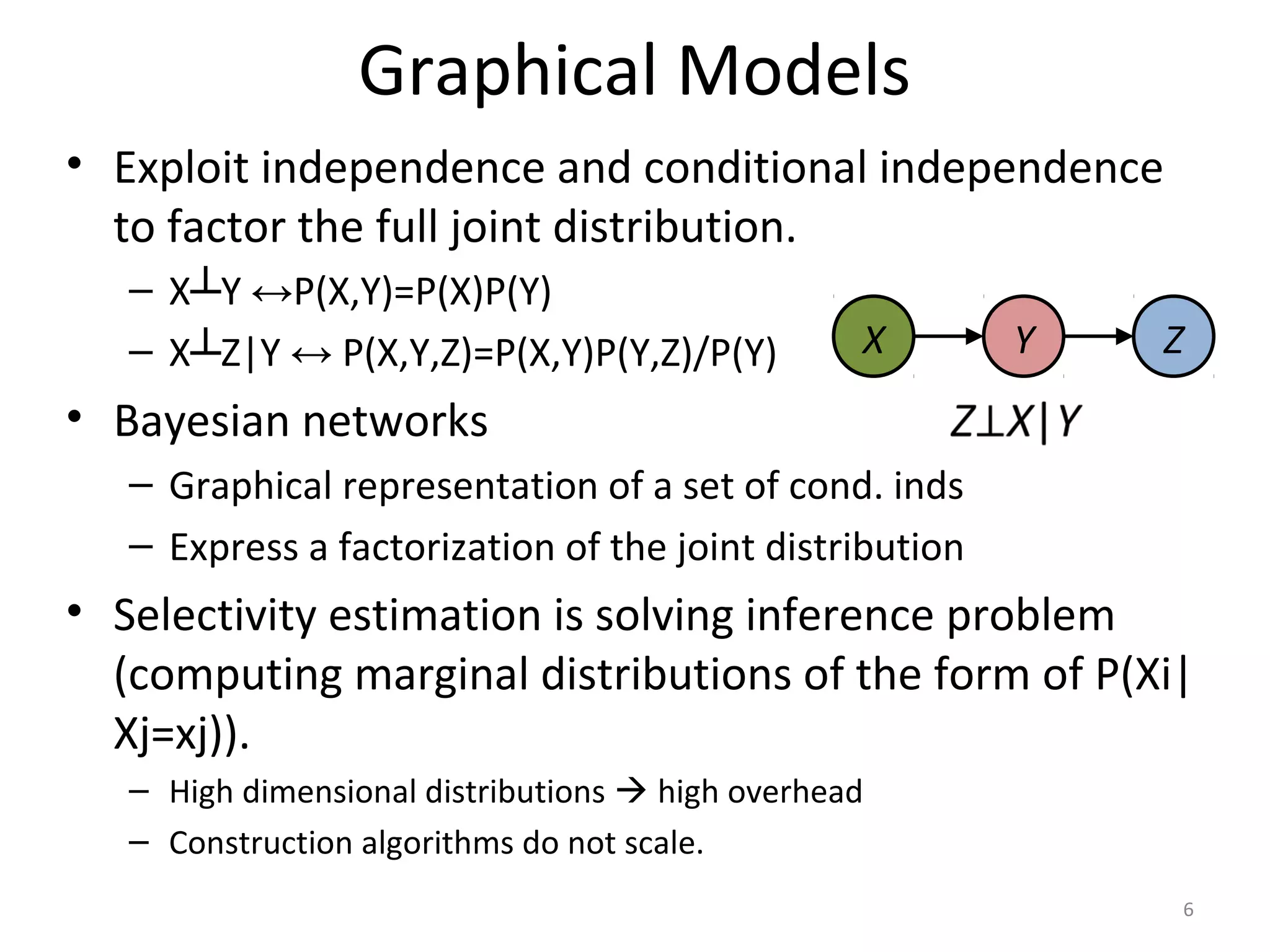
![Independence Assumption
|L’| = Pr(eprice in [e1,e2]) |L|
|O’| = Pr(tprice in [t1,t2]) |O|
|L’O’| = Pr(l_orderkey=o_orderkey)|L’||O’|
|L’O’| = Pr(l_orderkey=o_orderkey)
Pr(eprice in [e1,e2])
Pr(tprice in [t1,t2]) |L||O|
•Results to under-estimation of |L’O’|
wrong query plan, nested loop join.
•Can result in orders of magnitude slower
execution.
•Solution: estimate joint probabilities: |L’O’|
= Pr (l_orderkey=o_orderkey,
eprice in [e1,e2],
tprice in [t1,t2]) |L||O|
L O C
HJ
NLJ
σL σΟ σC
L’ O’ C’
L’O’
4
select c_name,c_address
from lineitem,orders,customer
where l_orderkey=o_orderkey and
o_custkey=c_custkey and
o_totalprice in [t1,t2] and
l_extendedprice in [e1,e2]
and c_acctbal in [b1,b2]](https://image.slidesharecdn.com/rsession16-1-150420154134-conversion-gate02/75/lightweight-graphical-models-for-selectivity-estimation-without-independance-assumption-4-2048.jpg)
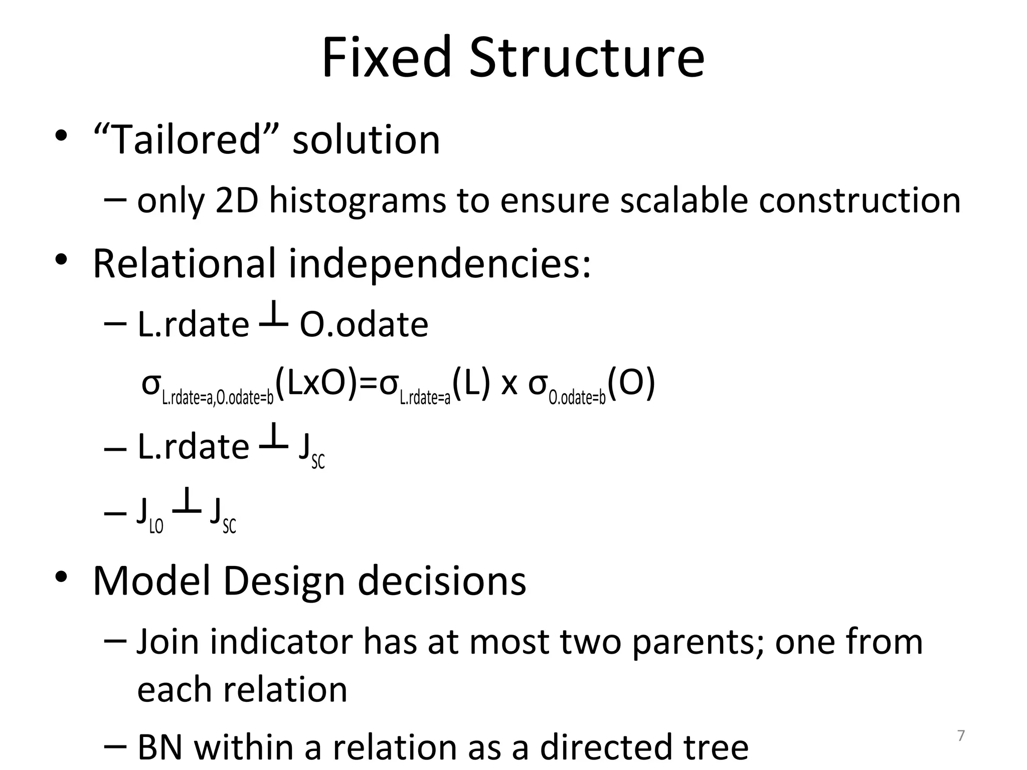
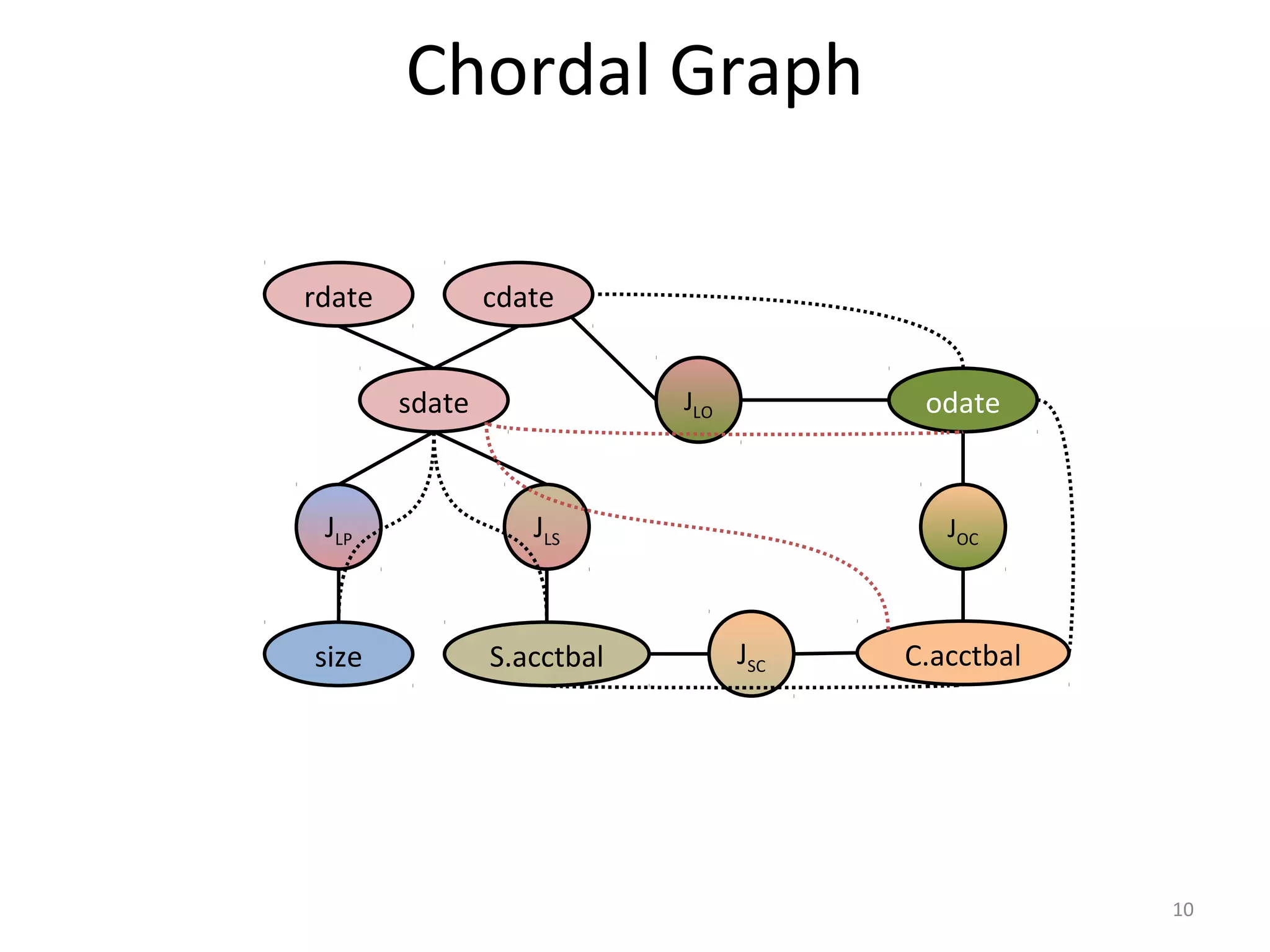
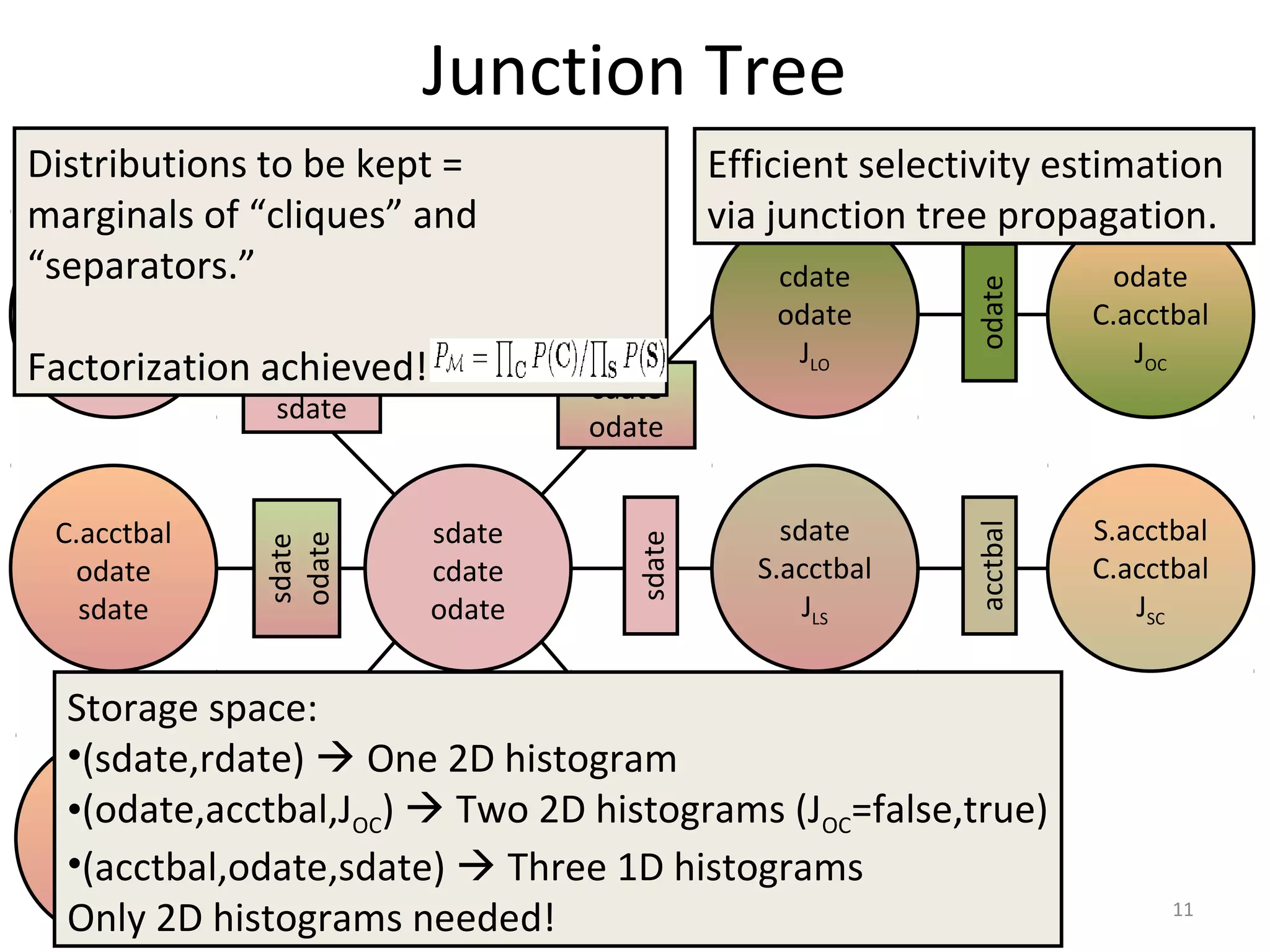
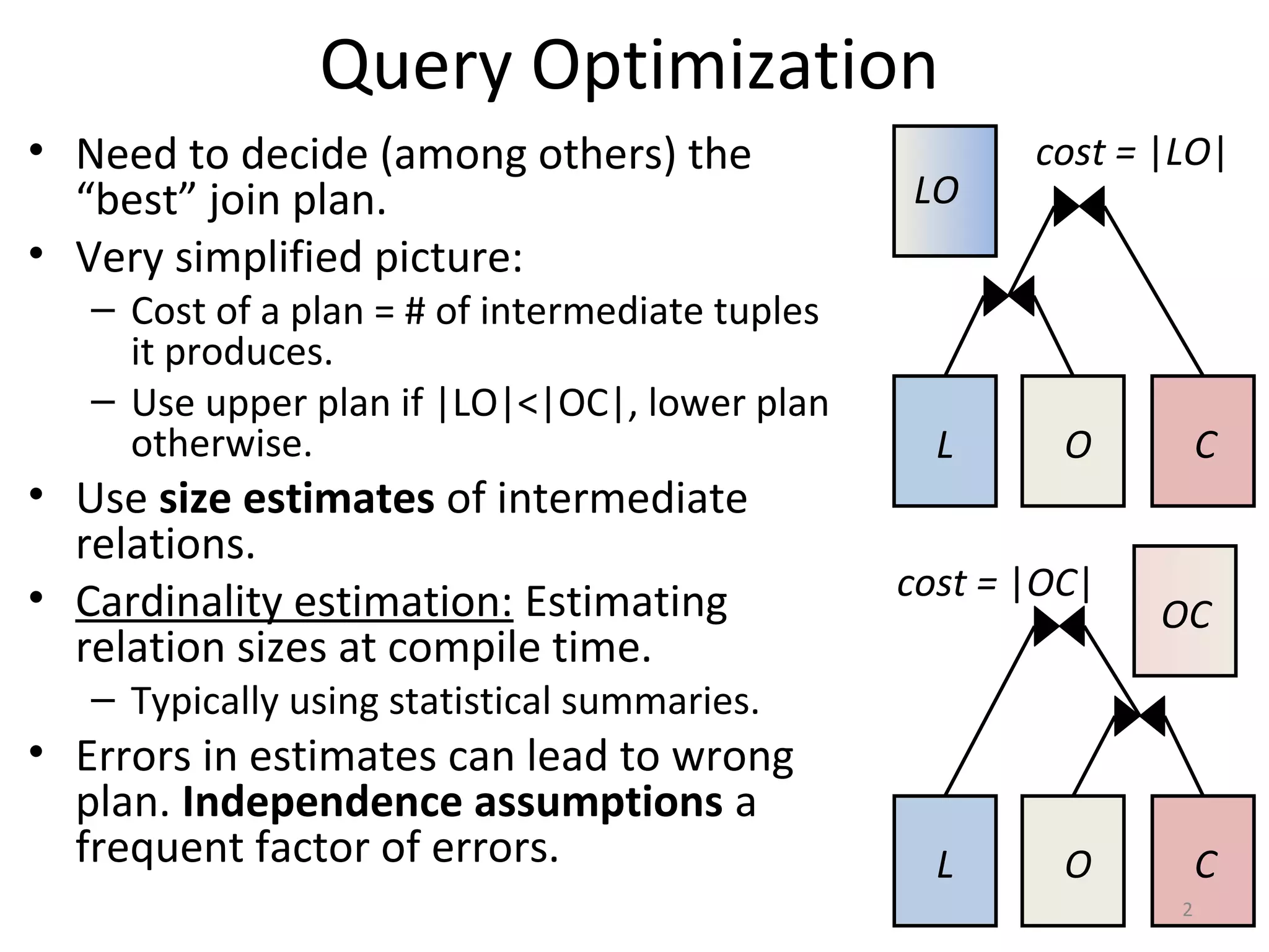
![Selectivity Estimation
sdate
cdate
odate
cdate
odate
JLO
odate
acctbal
JOC
cdate
odate
odate
Estimate
Pr(JLO=true,
JOC=true,
sdate<=“25/7/2011”,
acctbal<=200000)
φ2=P(cdate,odate,JLO)
φ3=P(odate,acctbal,JOC)
φ1=P(sdate,cdate,odate)
μ12=P(cdate,odate)
μ23=P(odate)
1. Substitute
φ1
*
(cdate,odate)=
φ1[sdate<=“25/7/2011”]
φ2
*
(cdate,odate)=
φ2[JLO=true]
φ3
*
(odate)=
φ3[JOC=true,acctbal<=200000]
2. Multiply
φ12
*
(cdate,odate)=
φ1
*
φ2
*
/μ12
3. Marginalize
φ12
**
(odate)=
Σcdateφ12
*
4. Multiply
φ123
*
(odate)=
φ12
**
φ3
*
/μ23
5. Return
Σodateφ123
*
13](https://image.slidesharecdn.com/rsession16-1-150420154134-conversion-gate02/75/lightweight-graphical-models-for-selectivity-estimation-without-independance-assumption-13-2048.jpg)
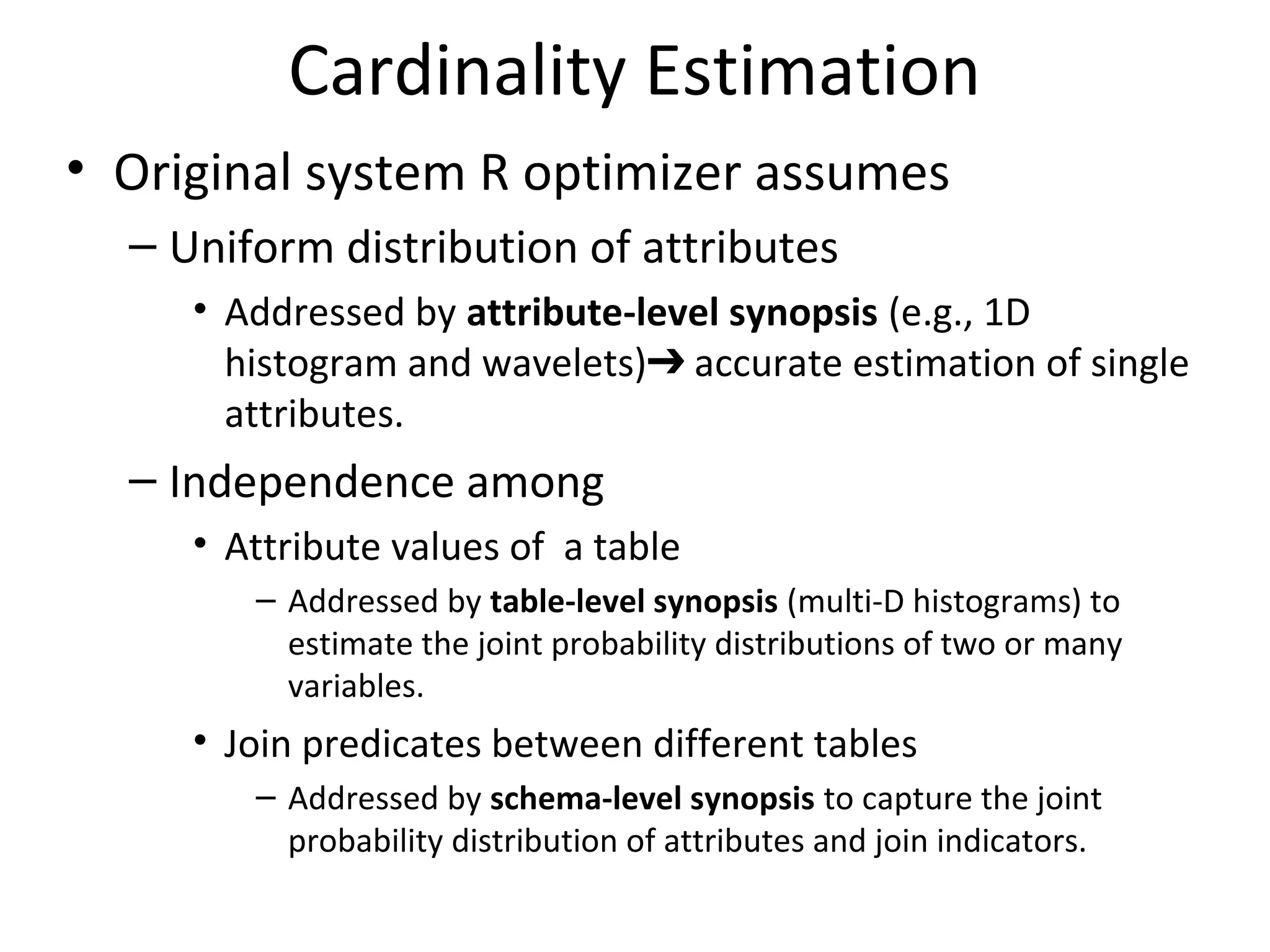
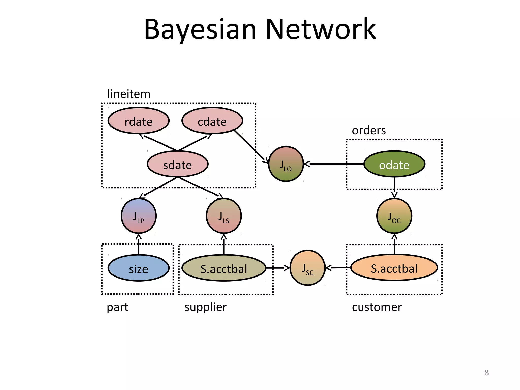
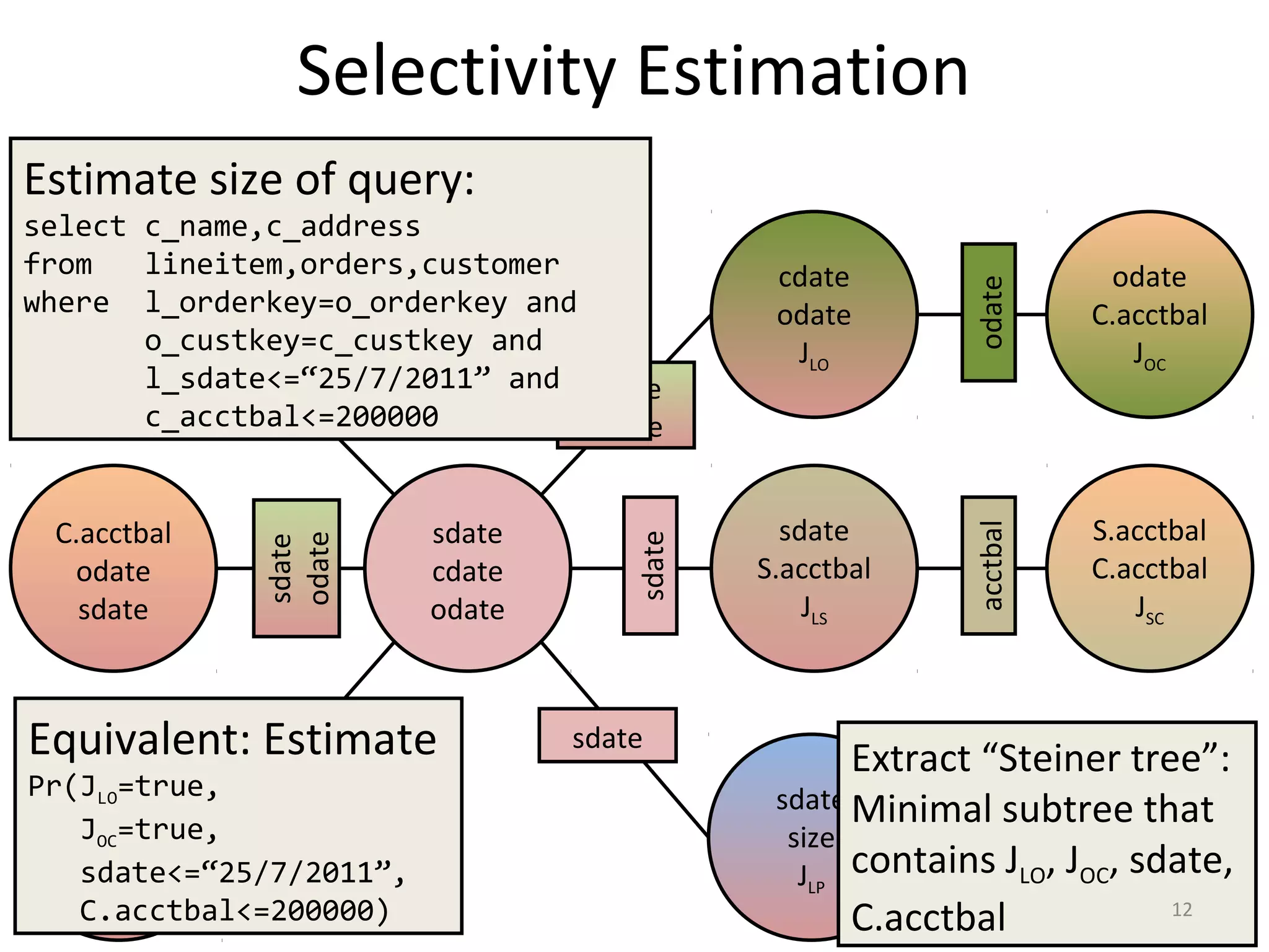
![Impact of Capturing Correlations
select c_name,c_address
from lineitem,orders,customer
where l_orderkey=o_orderkey and o_custkey=c_custkey
and o_tprice in [t1,t2] and l_eprice in [e1,e2]
and c_acctbal in [b1,b2]
Avoid under-estimation
by capturing the price
correlation.
Estimates very close to
reality.
Optimizer picks different
plan than default PGSQL.
Huge impact in
execution time.
Can do selectivity
estimation efficiently.
Optimization time in
the range of 10s of
milliseconds
Cost of plans (intermediate tuples)
Execution & optimization times
15](https://image.slidesharecdn.com/rsession16-1-150420154134-conversion-gate02/75/lightweight-graphical-models-for-selectivity-estimation-without-independance-assumption-15-2048.jpg)
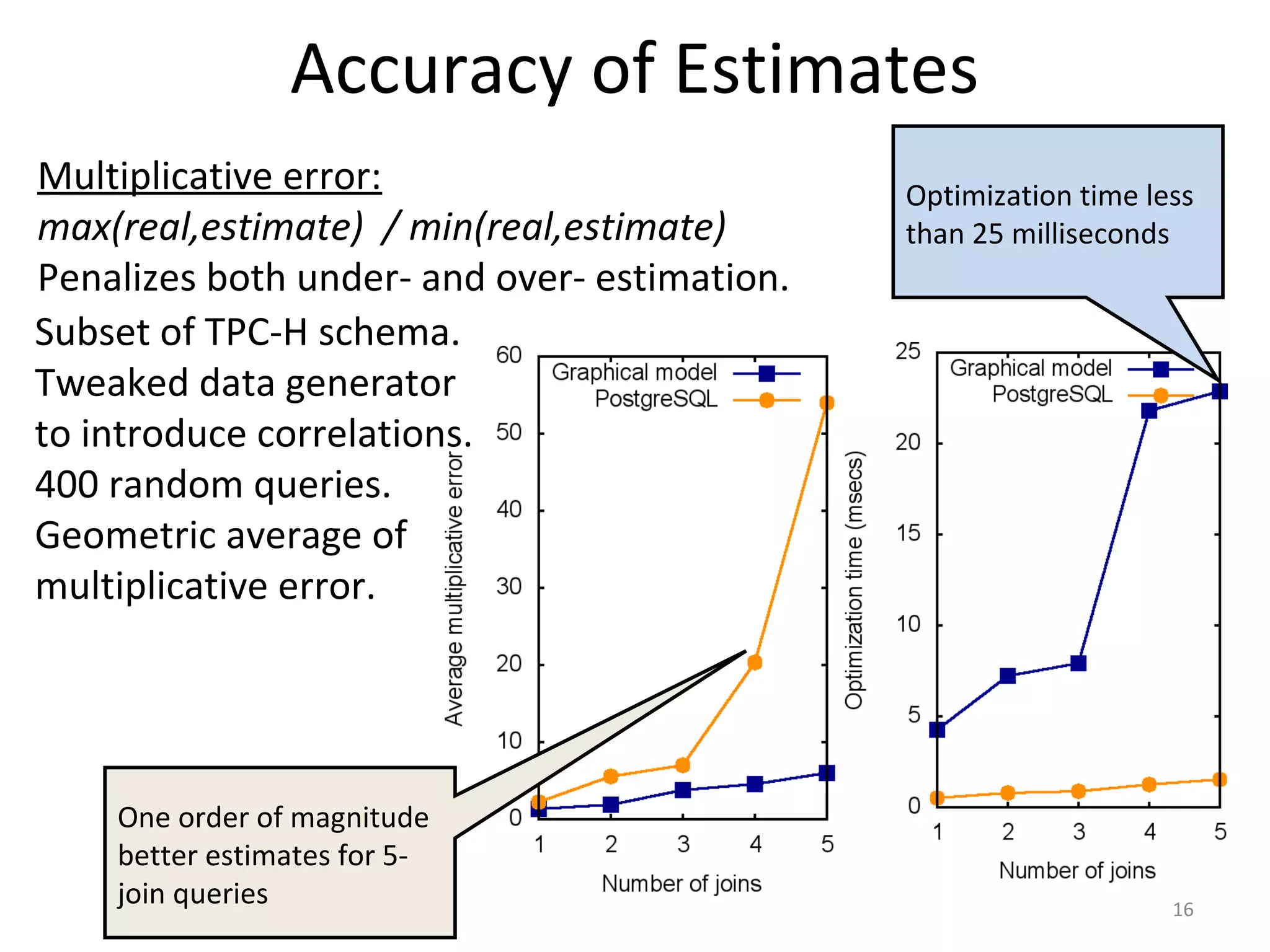

The document presents a technique for selectivity estimation in query optimization without assuming independence between attributes. It uses lightweight graphical models, specifically a junction tree, to capture correlations and approximate the joint probability distribution over relevant variables. This avoids the independence assumptions made by traditional optimizers that can lead to errors in cardinality estimates and suboptimal query plans. The graphical models are implemented within PostgreSQL to provide selectivity estimates with an order of magnitude better accuracy compared to the default PostgreSQL estimates, while keeping optimization time low.


![[ICIST 2013] A Probabilistic Relational Data Model for Uncertain Information](https://cdn.slidesharecdn.com/ss_thumbnails/aprobabilisticrelationaldatamodelforuncertaininformationv3-130330171529-phpapp02-thumbnail.jpg?width=640&height=640&fit=bounds)