Financial markets
modeling in R

Arbuzov V.

Perm State National Research
University

arbuzov@prognoz.ru
20 November 2013

Perm R group
r-group.mifit.ru

ITE.LAB “MathEconomics” Open Course
Russia, Perm, 20 November 2013

workshop
Basic knowledgement
about R
3

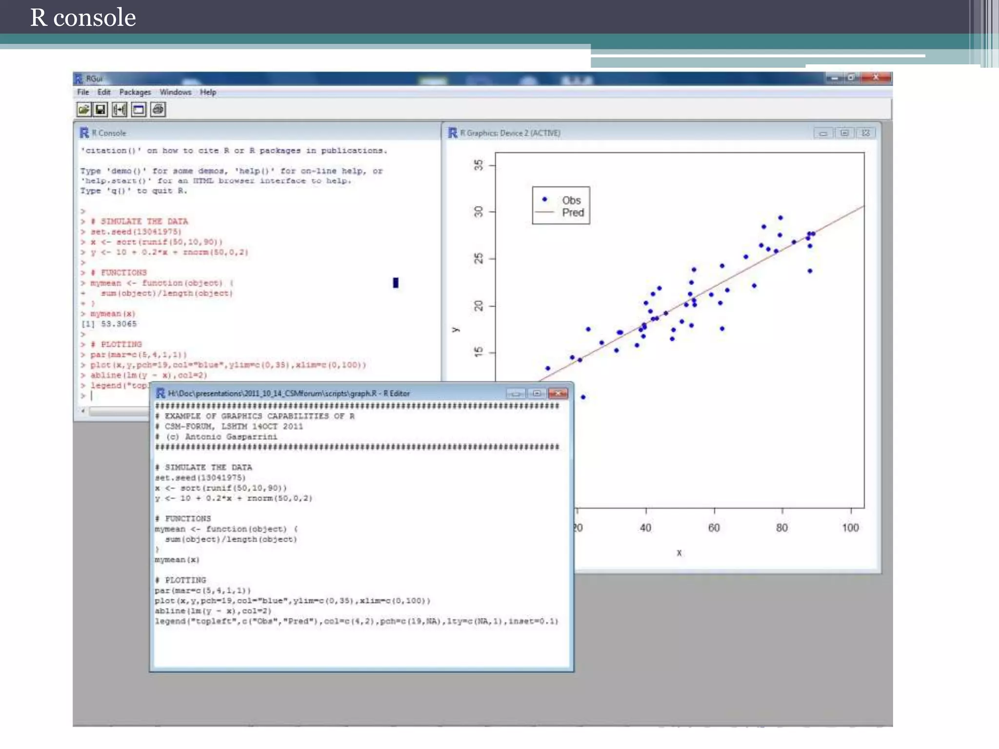
R console
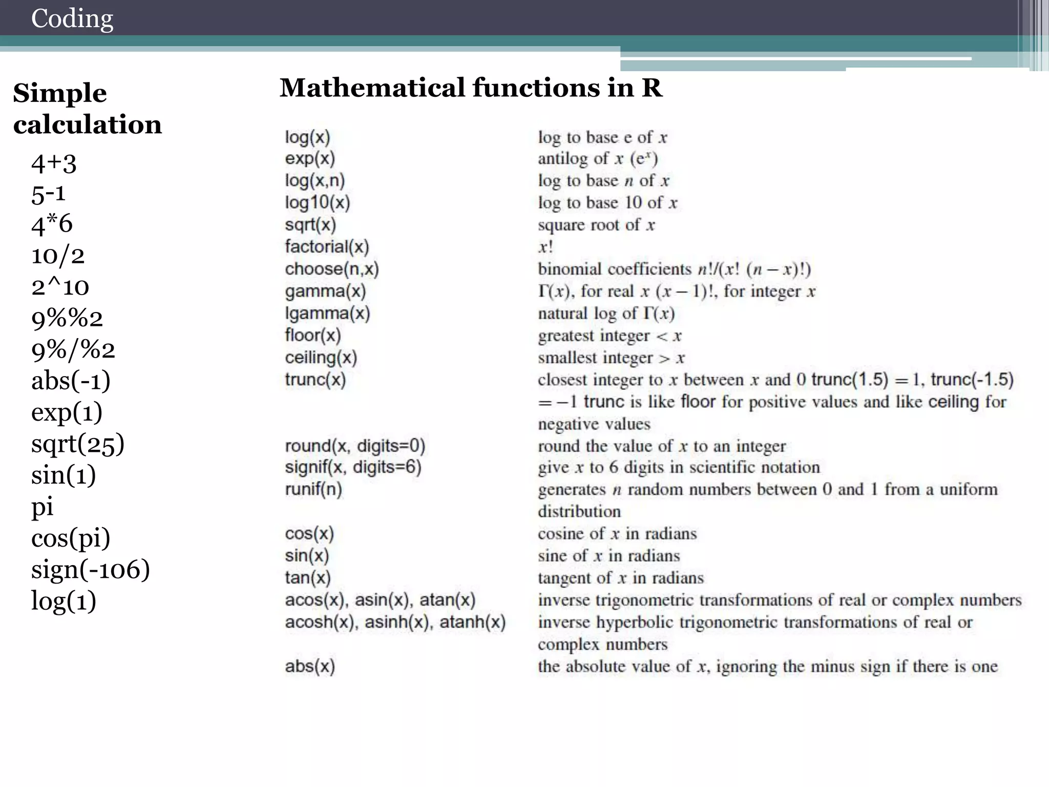
Coding
Simple
calculation
4+3
5-1
4*6
10/2
2^10
9%%2
9%/%2
abs(-1)
exp(1)
sqrt(25)
sin(1)
pi
cos(pi)
sign(-106)
log(1)

Mathematical functions in R
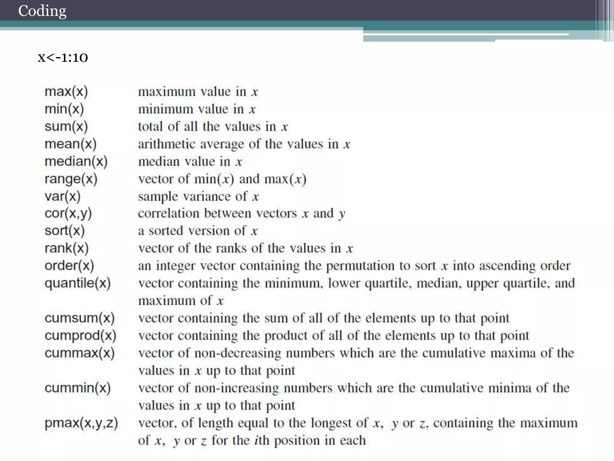
Coding
x<-1:10
Coding
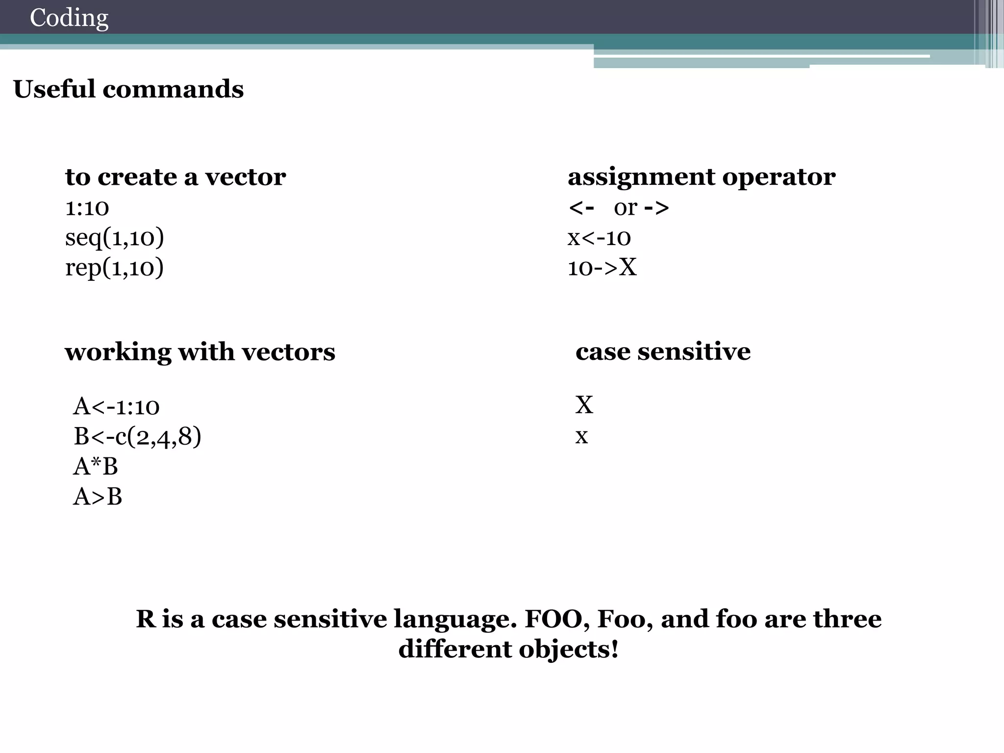
Useful commands
to create a vector
1:10
seq(1,10)
rep(1,10)
working with vectors
A<-1:10
B<-c(2,4,8)
A*B
A>B

assignment operator
<- or ->
x<-10
10->X
case sensitive
X
x

R is a case sensitive language. FOO, Foo, and foo are three
different objects!
Coding

Matrix
y <- matrix(nrow=2,ncol=2)
y[1,1] <- 1
y[2,1] <- 2
y[1,2] <- 3
y[2,2] <- 4
x <- matrix(1:4, 2, 2)

A matrix is a vector
with two additional
attributes: the
number of rows and
the
number of columns

Matrix Operations
x %*% y
x* y
3*y
x+y
x+3
x[,2]
x[1,]
rbind(x,y)->z
cbind(x,y)
z[1:2,]
z[z[,1]>1,]
z[which(z[,1]>1),1]
Coding
Data Frame

List

kids <- c("Jack","Jill")
ages <- c(12,10)
d <- data.frame(kids,ages)
d[1,]
d[,1]
d[[1]]

j <- list(name="Joe", salary=55000, union=T)
j$salary
j[["salary"]]
j[[2]]
j$name [2]<-”Poll”
j$salary[2]<-10000
j$union [2]<-”F”
Arrays
In contrast to a
vector, in which all
elements
must be of the same
mode, R’s list
structure can
combine objects of
different
types.

my.array <- array(1:24, dim=c(3,4,2))

a data frame is like a
matrix, with a two-dimensional rowsandcolumns
structure. However, it differs from
a matrix in that each column may have a
different
mode.
Coding
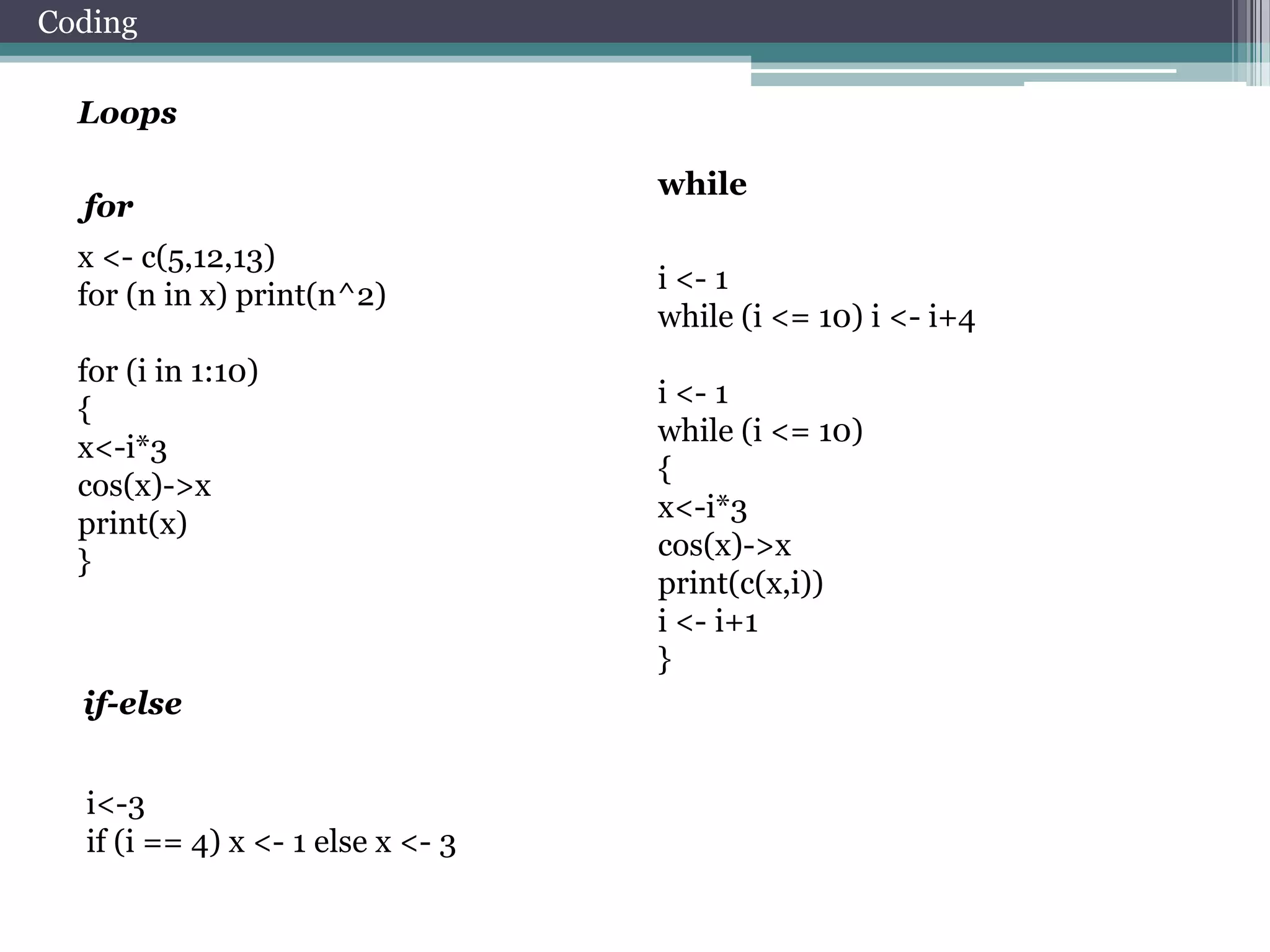
Loops
for
x <- c(5,12,13)
for (n in x) print(n^2)

for (i in 1:10)
{
x<-i*3
cos(x)->x
print(x)
}

if-else
i<-3
if (i == 4) x <- 1 else x <- 3

while
i <- 1
while (i <= 10) i <- i+4
i <- 1
while (i <= 10)
{
x<-i*3
cos(x)->x
print(c(x,i))
i <- i+1
}
Import/Export data
Import from text files or csv
mydata <read.table("d:/my.data.txt", header=TRUE
,
sep=",")
Import from Excel
library(xlsx)
mydata<-read.xlsx("d:/my.data.xlsx",1)
Exporting Data
write.table(mydata, "c:/mydata.txt", sep="t")

write.xlsx(mydata, "c:/mydata.xls")
Import/Export Data to clipboard
read.table("clipboard",sep="t")
write.table(arg1,"clipboard",sep="t")

rb <- function(arg1){read.table("clipboard",sep="t")}

P.S. cb <- function(arg1){write.table(arg1,"clipboard",sep="t")}
Basic Graphs

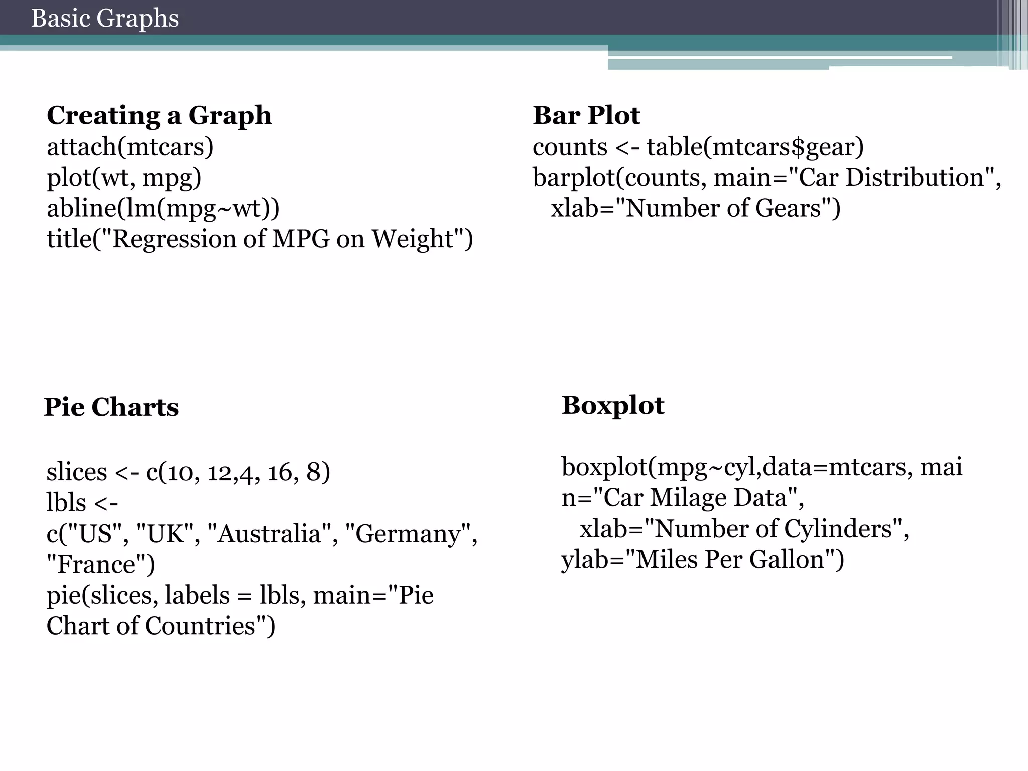
Creating a Graph
attach(mtcars)
plot(wt, mpg)
abline(lm(mpg~wt))
title("Regression of MPG on Weight")

Bar Plot
counts <- table(mtcars$gear)
barplot(counts, main="Car Distribution",
xlab="Number of Gears")

Pie Charts

Boxplot

slices <- c(10, 12,4, 16, 8)
lbls <c("US", "UK", "Australia", "Germany",
"France")
pie(slices, labels = lbls, main="Pie
Chart of Countries")

boxplot(mpg~cyl,data=mtcars, mai
n="Car Milage Data",
xlab="Number of Cylinders",
ylab="Miles Per Gallon")
Advanced
knowledgement
about R
Select data from matrix
x <- matrix(0,50,2)
x[,1]
x[1,]
x[,1]<-rnorm(50)
x
x[1,]<-rnorm(2)
x
x <- matrix(rnorm(100),50,2)
x[which(x[,1]>0),]
Operators
and
&
or
|
Distributions
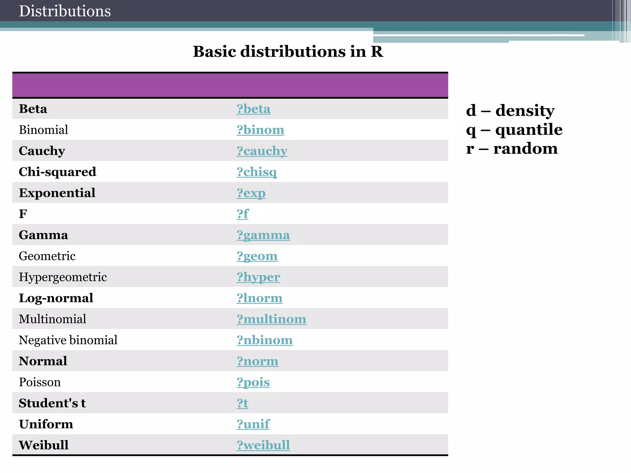
Basic distributions in R

Beta

?beta

Binomial

?binom

Cauchy

?cauchy

Chi-squared

?chisq

Exponential

?exp

F

?f

Gamma

?gamma

Geometric

?geom

Hypergeometric

?hyper

Log-normal

?lnorm

Multinomial

?multinom

Negative binomial

?nbinom

Normal

?norm

Poisson

?pois

Student's t

?t

Uniform

?unif

Weibull

?weibull

d – density
q – quantile
r – random
Distributions

Plot density of chosen distribution…

x <- seq(-4, 4, length=100)
dx <- d?????(x)
plot(x, hx, type=“l”)

Generate random variables of chosen
distribution …

x<-rnorm(1000)
Distributions
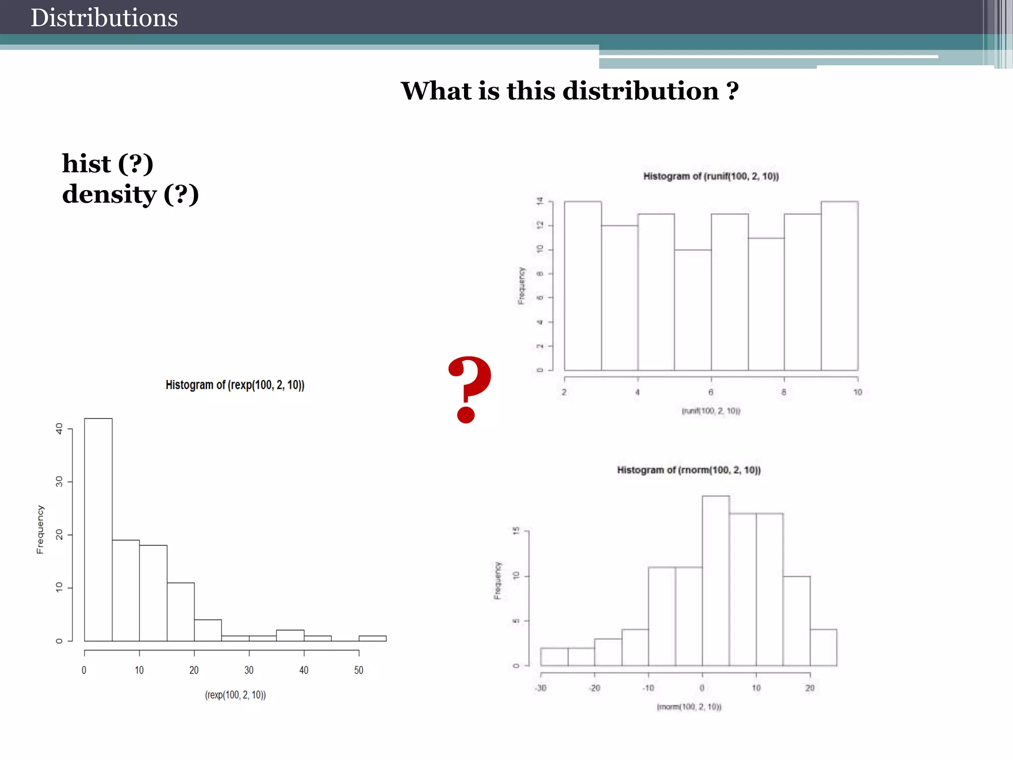
What is this distribution ?
hist (?)
density (?)

?
Estimation of parameters
Let’s estimate parameters of
chosen distribution….
library(MASS)
fitdistr(x,"normal")

params<-fitdistr(x,"normal")$estimate
Compare theoretical and empirical
distributions…
hist(x, freq = FALSE,ylim=c(0,0.4))
curve(dnorm(x, params[1], params[2]), col = 2, add = TRUE)
Correlations

y<-rnorm(1000)
cor(x,y)
cor(x,y, ,method = ?????)
acf(y)
Linear least-squares method

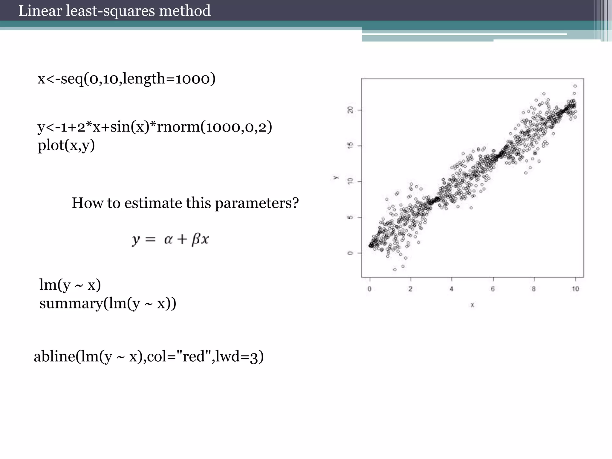
x<-seq(0,10,length=1000)
y<-1+2*x+sin(x)*rnorm(1000,0,2)
plot(x,y)

How to estimate this parameters?

lm(y ~ x)
summary(lm(y ~ x))
abline(lm(y ~ x),col="red",lwd=3)
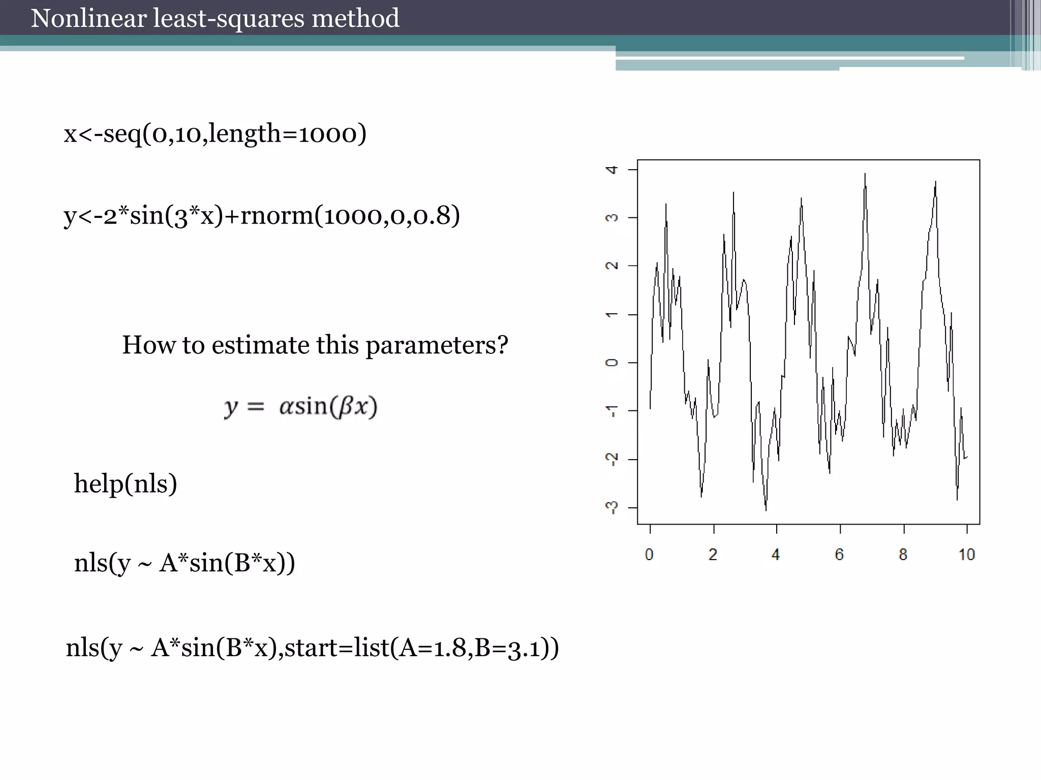
Nonlinear least-squares method

x<-seq(0,10,length=1000)
y<-2*sin(3*x)+rnorm(1000,0,0.8)

How to estimate this parameters?

help(nls)

nls(y ~ A*sin(B*x))
nls(y ~ A*sin(B*x),start=list(A=1.8,B=3.1))
Advanced graphics

Add few diagrams to graph

par(mfrow=c(2,2))
plot(rnorm(100),rbeta(100,12,1))
Add legend to graph

legend("topright", inset=.05, title="legend",
c("4","6","8"), horiz=TRUE)
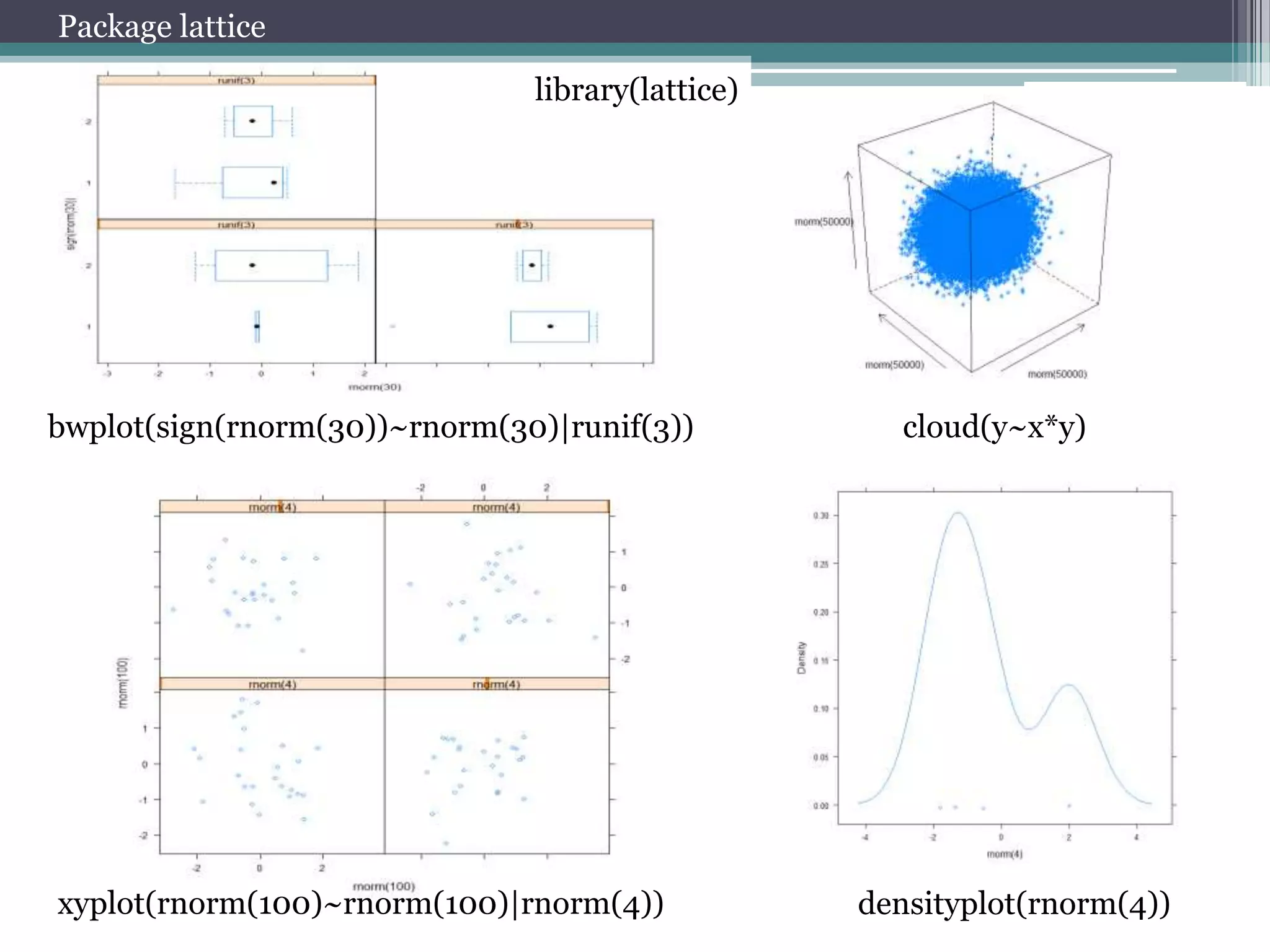
Package lattice
library(lattice)

bwplot(sign(rnorm(30))~rnorm(30)|runif(3))

xyplot(rnorm(100)~rnorm(100)|rnorm(4))

cloud(y~x*y)

densityplot(rnorm(4))
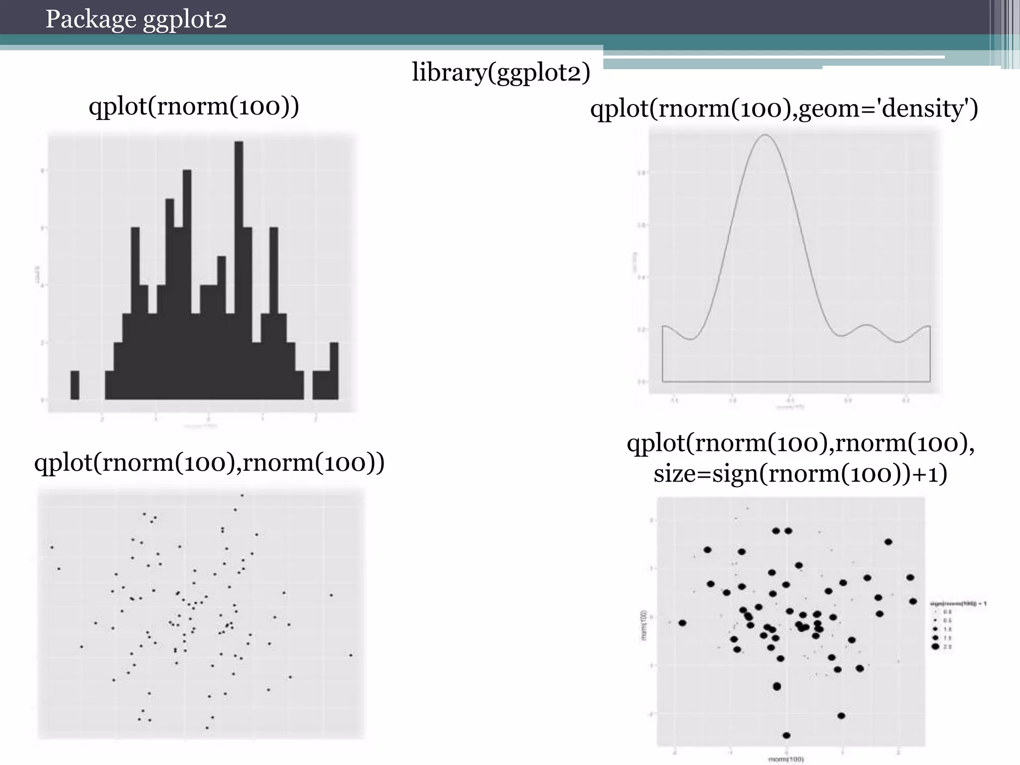
Package ggplot2
qplot(rnorm(100))

qplot(rnorm(100),rnorm(100))

library(ggplot2)
qplot(rnorm(100),geom='density')

qplot(rnorm(100),rnorm(100),
size=sign(rnorm(100))+1)
Download Data
Package quantmod

Package rusquant

getSymbols("GOOG",src="yahoo",
from = "2007-01-01“, to =
Sys.Date())

getSymbols("SPFB.RTS", from="2011-0101", src="Finam“, period="hour"
, auto.assign=FALSE)

getSymbols("USD/EUR",src="oanda")

1min, 5min, 10min, 15min,
30min, hour, day, week, month
Working with package quantmod

Data visualization

Add technical indicators

barChart(AAPL)
candleChart(AAPL,multi.col=TRUE,theme="white")

addMACD()

chartSeries(AAPL,up.col='white',dn.col='blue')

addBBands()

Select data

AAPL['2007']
AAPL['2007-03/2007']
AAPL['/2007']
AAPL['2007-01-03']

Data management

to.weekly(AAPL)
to.monthly(AAPL)
dailyReturn(AAPL)
weeklyReturn(AAPL)
monthlyReturn(AAPL)
Load Data from Database
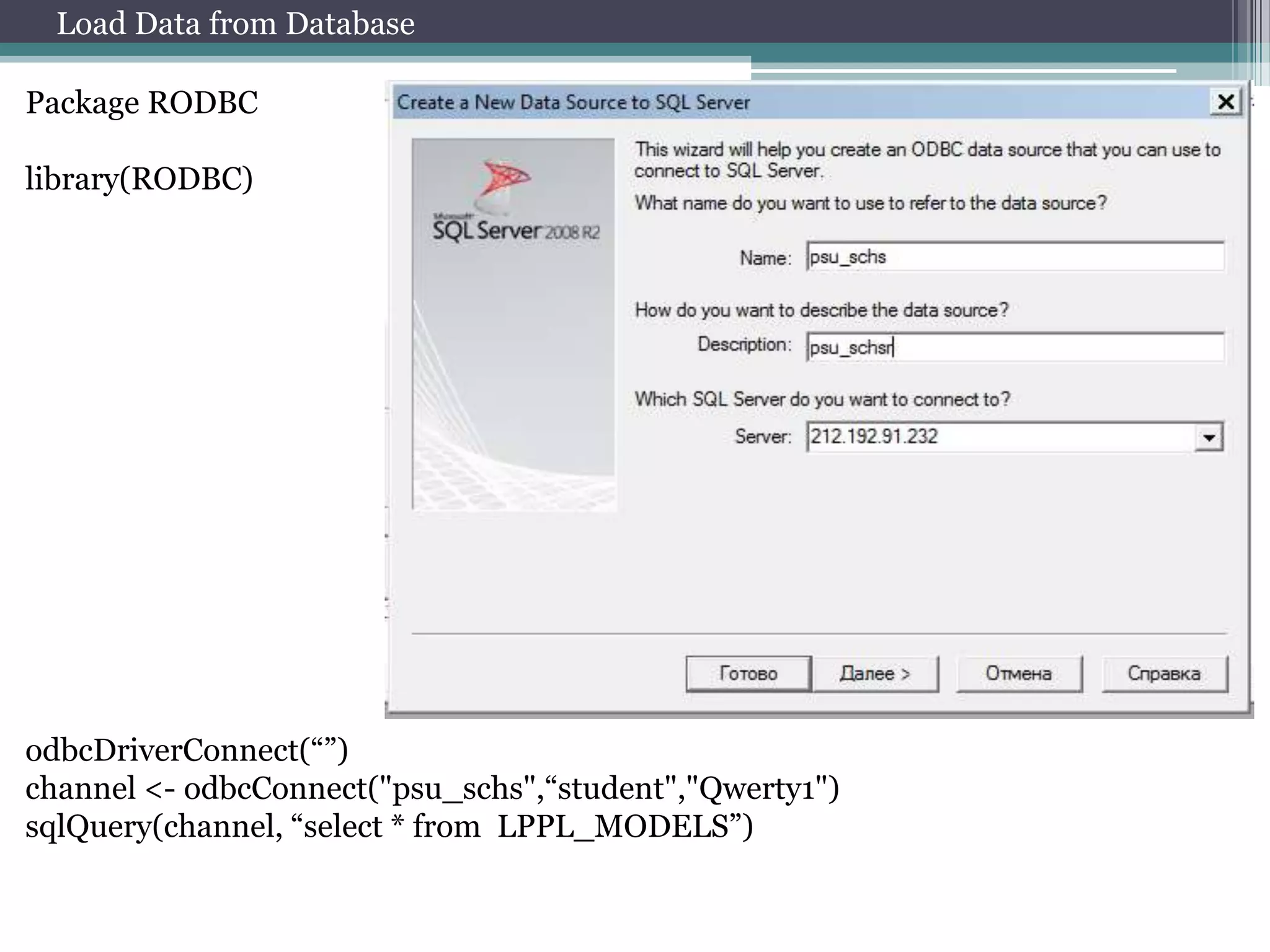
Package RODBC
library(RODBC)

odbcDriverConnect(“”)
channel <- odbcConnect("psu_schs",“student","Qwerty1")
sqlQuery(channel, “select * from LPPL_MODELS”)
Practice
Practice № 1. Working with data

1. AAPL
2. BAC
3. GOOG
4. GE
5. GM
6. PG
7. JNJ
8. JPM
9. LNKD
10. MSFT
11. NOK
12. IBM
13. AMZN
14. V

TASK:
a. Download Data of your instrument
b. Plot price
c. Add technical indicators
d. Calculate price returns

Commands to help :
barChart(AAPL)
chartSeries(AAPL,up.col='white',dn.col='blue')
AAPL['2007-03/2007']
addMACD()
dailyReturn(AAPL)
Practice № 2. Distribution of price returns

1. AAPL
2. BAC
3. GOOG
4. GE
5. GM
6. PG
7. JNJ
8. JPM
9. LNKD
10. MSFT
11. NOK
12. IBM
13. AMZN
14. V

TASK :
a. Download Data of your instrument
b. Calculate returns of close prices
c. Plot density of distribution
d. Estimate parameters of distribution
e. Plot in one graph empirical and theoretical
distributions

Commands to help :
getSymbols("AAPL", auto.assign=FALSE)
library(MASS)
fitdistr(x,"normal")
hist(x)
density(x)
curve(dnorm(x, params[1], params[2]), col = 2, add = TRUE)
Practice № 3. Estimation of correlation

1. AAPL
2. BAC
3. GOOG
4. GE
5. GM
6. PG
7. JNJ
8. JPM
9. LNKD
10. MSFT
11. NOK
12. IBM
13. AMZN
14. V

TASK :
a. Download Index Data (ticker: “MICEX”)
b. Download Data of your instrument
c. Calculate returns of close prices
d. Calculate correlation of returns
e. Calculate correlation of returns in 2012 year
f. Calculate correlation of returns in 2008 year
g. Calculate autocorrelation function of returns
Commands to help :
getSymbols(" MICEX ",
src="Finam", period="day" , auto.assign=FALSE)

AAPL['2007']
AAPL['2007-03/2007']
AAPL['/2007']
AAPL['2007-01-03']
Practice № 4. Volatility estimation

1. AAPL
2. BAC
3. GOOG
4. GE
5. GM
6. PG
7. JNJ
8. JPM
9. LNKD
10. MSFT
11. NOK
12. IBM
13. AMZN
14. V

TASK :
a. Download Data of your instrument
b. Calculate returns of close prices
c. Plot clusterization of volatility
d. Estimate model garch
e. garchFit(data=x) @sigma.t

Commands to help :
AAPL['2007']
AAPL['2007-03/2007']
AAPL['/2007']
AAPL['2007-01-03']
The practical task №5. Calculation of VaR

1. AAPL
2. BAC
3. GOOG
4. GE
5. GM
6. PG
7. JNJ
8. JPM
9. LNKD
10. MSFT
11. NOK
12. IBM
13. AMZN
14. V

TASK :
a. Download Data of your instrument
b. Calculate returns of close prices
c. Calculate historical VaR
d. Calculate parametric VaR
e. library(PerformanceAnalytics)
f. help(VaR)

Commands to help :
quantile(x,0.95, na.rm=TRUE)
AAPL['2007']
AAPL['2007-03/2007']
AAPL['/2007']
AAPL['2007-01-03']
The practical task № 6. Estimate LPPL model
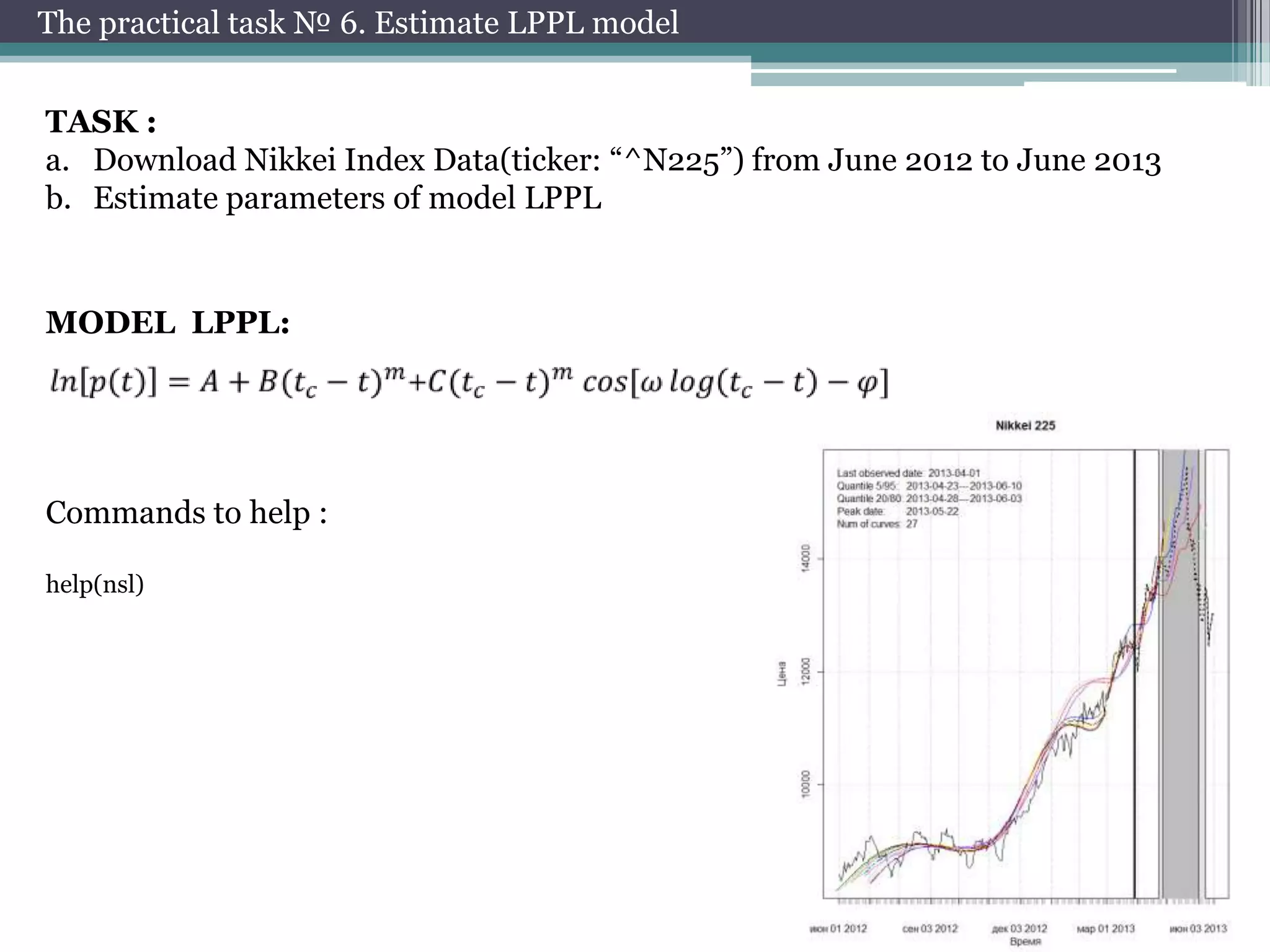
TASK :
a. Download Nikkei Index Data(ticker: “^N225”) from June 2012 to June 2013
b. Estimate parameters of model LPPL

MODEL LPPL:

Commands to help :
help(nsl)
Q&A

arbuzov@prognoz.ru

Seminar psu 20.10.2013

  • 1.
    Financial markets modeling inR Arbuzov V. Perm State National Research University arbuzov@prognoz.ru 20 November 2013 Perm R group r-group.mifit.ru ITE.LAB “MathEconomics” Open Course Russia, Perm, 20 November 2013 workshop
  • 2.
  • 3.
  • 4.
  • 5.
  • 6.
    Coding Useful commands to createa vector 1:10 seq(1,10) rep(1,10) working with vectors A<-1:10 B<-c(2,4,8) A*B A>B assignment operator <- or -> x<-10 10->X case sensitive X x R is a case sensitive language. FOO, Foo, and foo are three different objects!
  • 7.
    Coding Matrix y <- matrix(nrow=2,ncol=2) y[1,1]<- 1 y[2,1] <- 2 y[1,2] <- 3 y[2,2] <- 4 x <- matrix(1:4, 2, 2) A matrix is a vector with two additional attributes: the number of rows and the number of columns Matrix Operations x %*% y x* y 3*y x+y x+3 x[,2] x[1,] rbind(x,y)->z cbind(x,y) z[1:2,] z[z[,1]>1,] z[which(z[,1]>1),1]
  • 8.
    Coding Data Frame List kids <-c("Jack","Jill") ages <- c(12,10) d <- data.frame(kids,ages) d[1,] d[,1] d[[1]] j <- list(name="Joe", salary=55000, union=T) j$salary j[["salary"]] j[[2]] j$name [2]<-”Poll” j$salary[2]<-10000 j$union [2]<-”F” Arrays In contrast to a vector, in which all elements must be of the same mode, R’s list structure can combine objects of different types. my.array <- array(1:24, dim=c(3,4,2)) a data frame is like a matrix, with a two-dimensional rowsandcolumns structure. However, it differs from a matrix in that each column may have a different mode.
  • 9.
    Coding Loops for x <- c(5,12,13) for(n in x) print(n^2) for (i in 1:10) { x<-i*3 cos(x)->x print(x) } if-else i<-3 if (i == 4) x <- 1 else x <- 3 while i <- 1 while (i <= 10) i <- i+4 i <- 1 while (i <= 10) { x<-i*3 cos(x)->x print(c(x,i)) i <- i+1 }
  • 10.
    Import/Export data Import fromtext files or csv mydata <read.table("d:/my.data.txt", header=TRUE , sep=",") Import from Excel library(xlsx) mydata<-read.xlsx("d:/my.data.xlsx",1) Exporting Data write.table(mydata, "c:/mydata.txt", sep="t") write.xlsx(mydata, "c:/mydata.xls") Import/Export Data to clipboard read.table("clipboard",sep="t") write.table(arg1,"clipboard",sep="t") rb <- function(arg1){read.table("clipboard",sep="t")} P.S. cb <- function(arg1){write.table(arg1,"clipboard",sep="t")}
  • 11.
    Basic Graphs Creating aGraph attach(mtcars) plot(wt, mpg) abline(lm(mpg~wt)) title("Regression of MPG on Weight") Bar Plot counts <- table(mtcars$gear) barplot(counts, main="Car Distribution", xlab="Number of Gears") Pie Charts Boxplot slices <- c(10, 12,4, 16, 8) lbls <c("US", "UK", "Australia", "Germany", "France") pie(slices, labels = lbls, main="Pie Chart of Countries") boxplot(mpg~cyl,data=mtcars, mai n="Car Milage Data", xlab="Number of Cylinders", ylab="Miles Per Gallon")
  • 12.
  • 13.
    Select data frommatrix x <- matrix(0,50,2) x[,1] x[1,] x[,1]<-rnorm(50) x x[1,]<-rnorm(2) x x <- matrix(rnorm(100),50,2) x[which(x[,1]>0),] Operators and & or |
  • 14.
    Distributions Basic distributions inR Beta ?beta Binomial ?binom Cauchy ?cauchy Chi-squared ?chisq Exponential ?exp F ?f Gamma ?gamma Geometric ?geom Hypergeometric ?hyper Log-normal ?lnorm Multinomial ?multinom Negative binomial ?nbinom Normal ?norm Poisson ?pois Student's t ?t Uniform ?unif Weibull ?weibull d – density q – quantile r – random
  • 15.
    Distributions Plot density ofchosen distribution… x <- seq(-4, 4, length=100) dx <- d?????(x) plot(x, hx, type=“l”) Generate random variables of chosen distribution … x<-rnorm(1000)
  • 16.
    Distributions What is thisdistribution ? hist (?) density (?) ?
  • 17.
    Estimation of parameters Let’sestimate parameters of chosen distribution…. library(MASS) fitdistr(x,"normal") params<-fitdistr(x,"normal")$estimate Compare theoretical and empirical distributions… hist(x, freq = FALSE,ylim=c(0,0.4)) curve(dnorm(x, params[1], params[2]), col = 2, add = TRUE)
  • 18.
  • 19.
    Linear least-squares method x<-seq(0,10,length=1000) y<-1+2*x+sin(x)*rnorm(1000,0,2) plot(x,y) Howto estimate this parameters? lm(y ~ x) summary(lm(y ~ x)) abline(lm(y ~ x),col="red",lwd=3)
  • 20.
    Nonlinear least-squares method x<-seq(0,10,length=1000) y<-2*sin(3*x)+rnorm(1000,0,0.8) Howto estimate this parameters? help(nls) nls(y ~ A*sin(B*x)) nls(y ~ A*sin(B*x),start=list(A=1.8,B=3.1))
  • 21.
    Advanced graphics Add fewdiagrams to graph par(mfrow=c(2,2)) plot(rnorm(100),rbeta(100,12,1)) Add legend to graph legend("topright", inset=.05, title="legend", c("4","6","8"), horiz=TRUE)
  • 22.
  • 23.
  • 24.
    Download Data Package quantmod Packagerusquant getSymbols("GOOG",src="yahoo", from = "2007-01-01“, to = Sys.Date()) getSymbols("SPFB.RTS", from="2011-0101", src="Finam“, period="hour" , auto.assign=FALSE) getSymbols("USD/EUR",src="oanda") 1min, 5min, 10min, 15min, 30min, hour, day, week, month
  • 25.
    Working with packagequantmod Data visualization Add technical indicators barChart(AAPL) candleChart(AAPL,multi.col=TRUE,theme="white") addMACD() chartSeries(AAPL,up.col='white',dn.col='blue') addBBands() Select data AAPL['2007'] AAPL['2007-03/2007'] AAPL['/2007'] AAPL['2007-01-03'] Data management to.weekly(AAPL) to.monthly(AAPL) dailyReturn(AAPL) weeklyReturn(AAPL) monthlyReturn(AAPL)
  • 26.
    Load Data fromDatabase Package RODBC library(RODBC) odbcDriverConnect(“”) channel <- odbcConnect("psu_schs",“student","Qwerty1") sqlQuery(channel, “select * from LPPL_MODELS”)
  • 27.
  • 28.
    Practice № 1.Working with data 1. AAPL 2. BAC 3. GOOG 4. GE 5. GM 6. PG 7. JNJ 8. JPM 9. LNKD 10. MSFT 11. NOK 12. IBM 13. AMZN 14. V TASK: a. Download Data of your instrument b. Plot price c. Add technical indicators d. Calculate price returns Commands to help : barChart(AAPL) chartSeries(AAPL,up.col='white',dn.col='blue') AAPL['2007-03/2007'] addMACD() dailyReturn(AAPL)
  • 29.
    Practice № 2.Distribution of price returns 1. AAPL 2. BAC 3. GOOG 4. GE 5. GM 6. PG 7. JNJ 8. JPM 9. LNKD 10. MSFT 11. NOK 12. IBM 13. AMZN 14. V TASK : a. Download Data of your instrument b. Calculate returns of close prices c. Plot density of distribution d. Estimate parameters of distribution e. Plot in one graph empirical and theoretical distributions Commands to help : getSymbols("AAPL", auto.assign=FALSE) library(MASS) fitdistr(x,"normal") hist(x) density(x) curve(dnorm(x, params[1], params[2]), col = 2, add = TRUE)
  • 30.
    Practice № 3.Estimation of correlation 1. AAPL 2. BAC 3. GOOG 4. GE 5. GM 6. PG 7. JNJ 8. JPM 9. LNKD 10. MSFT 11. NOK 12. IBM 13. AMZN 14. V TASK : a. Download Index Data (ticker: “MICEX”) b. Download Data of your instrument c. Calculate returns of close prices d. Calculate correlation of returns e. Calculate correlation of returns in 2012 year f. Calculate correlation of returns in 2008 year g. Calculate autocorrelation function of returns Commands to help : getSymbols(" MICEX ", src="Finam", period="day" , auto.assign=FALSE) AAPL['2007'] AAPL['2007-03/2007'] AAPL['/2007'] AAPL['2007-01-03']
  • 31.
    Practice № 4.Volatility estimation 1. AAPL 2. BAC 3. GOOG 4. GE 5. GM 6. PG 7. JNJ 8. JPM 9. LNKD 10. MSFT 11. NOK 12. IBM 13. AMZN 14. V TASK : a. Download Data of your instrument b. Calculate returns of close prices c. Plot clusterization of volatility d. Estimate model garch e. garchFit(data=x) @sigma.t Commands to help : AAPL['2007'] AAPL['2007-03/2007'] AAPL['/2007'] AAPL['2007-01-03']
  • 32.
    The practical task№5. Calculation of VaR 1. AAPL 2. BAC 3. GOOG 4. GE 5. GM 6. PG 7. JNJ 8. JPM 9. LNKD 10. MSFT 11. NOK 12. IBM 13. AMZN 14. V TASK : a. Download Data of your instrument b. Calculate returns of close prices c. Calculate historical VaR d. Calculate parametric VaR e. library(PerformanceAnalytics) f. help(VaR) Commands to help : quantile(x,0.95, na.rm=TRUE) AAPL['2007'] AAPL['2007-03/2007'] AAPL['/2007'] AAPL['2007-01-03']
  • 33.
    The practical task№ 6. Estimate LPPL model TASK : a. Download Nikkei Index Data(ticker: “^N225”) from June 2012 to June 2013 b. Estimate parameters of model LPPL MODEL LPPL: Commands to help : help(nsl)
  • 34.