Download as PDF, PPTX

![Matrix Games solver
The problem is to compute an x such that
Ax ≤ e, x ∈ S = {x ∈ Rn|e x = 1, x ≥ 0}
where
A is the payoff matrix
A = −A
Elements of A lie in [−1, 1]
∈ (0, 1]
n ≥ 8](https://image.slidesharecdn.com/designandimplementationofparallelan2-160331112955/85/Design-and-Implementation-of-Parallel-and-Randomized-Approximation-Algorithms-3-320.jpg)
![Matrix Games solver
Our solver returns
x ∈ Rn
, an optimal strategy vector for A
with probability ≥ 1/2
Time complexity
O( 1
2 log2
n) expected time on an n/ log n-processor [Khachiyan
et al. [5]] (we will refer it by GK)
Our solver takes O( 1
2 n log n) at most time on single processor](https://image.slidesharecdn.com/designandimplementationofparallelan2-160331112955/85/Design-and-Implementation-of-Parallel-and-Randomized-Approximation-Algorithms-4-320.jpg)
![Linear Programs solver
LP of the form
Packing:
max{|x| : Ax ≤ 1, x ≥ 0}
Covering:
min{|ˆx| : A ˆx ≥ 1, ˆx ≥ 0}
Note: Coefficients of xj ’s and bi ’s are one, for i = 1, 2, ..., r
and j = 1, 2, ..., c.
where
Elements of the constraint matrix A lie in [0, 1]r×c
r and c is number of rows and column respectively](https://image.slidesharecdn.com/designandimplementationofparallelan2-160331112955/85/Design-and-Implementation-of-Parallel-and-Randomized-Approximation-Algorithms-6-320.jpg)
![Linear Programs solver
Our solver returns
A (1 − 2 ) - approximate feasible primal-dual pair x and ˆx
|x | ≥ (1 − 2 )|ˆx | [Christos et al. [6]] (We will refer it by KY)
with probability at least 1 − 1/(rc)
∈ (0, 1]
Time complexity
Our solver takes O( 1
2 n log n) at most time on single processor](https://image.slidesharecdn.com/designandimplementationofparallelan2-160331112955/85/Design-and-Implementation-of-Parallel-and-Randomized-Approximation-Algorithms-7-320.jpg)
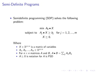
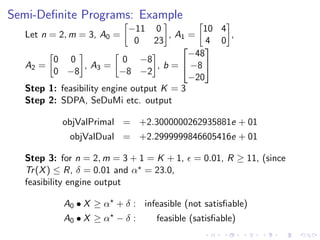
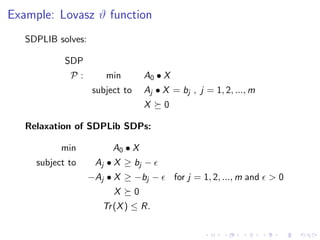
![Example: Lovasz ϑ function
Consider following SDP problems from SDPLIB 1.2 [2]
theta1, theta2 and theta3
Given a graph G = (V , E), the lovasz ϑ-function ϑ(G) on G
is the optimal value of the following SDP
max J • X
I • X = 1
∀{i, j} ∈ E : Eij • X = 0
X 0.
Where
I is identity matrix
J is matrix in which every entry is 1
For each edge {i, j} ∈ E, Eij is the matrix in which both the
(i, j)-th and (j, i)-th entries are 1, and every other entry is 0](https://image.slidesharecdn.com/designandimplementationofparallelan2-160331112955/85/Design-and-Implementation-of-Parallel-and-Randomized-Approximation-Algorithms-14-320.jpg)
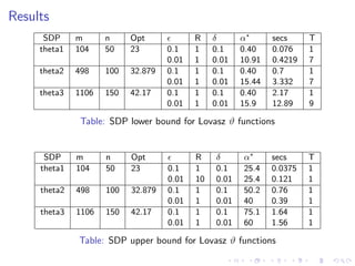


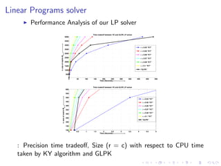
This document summarizes the design and implementation of parallel and randomized approximation algorithms for solving matrix games, linear programs, and semi-definite programs. It presents solvers for these problems that provide approximate solutions in sublinear or near-linear time. It analyzes the performance and precision-time tradeoffs of the solvers compared to other algorithms. It also provides examples of applying the SDP solver to approximate the Lovasz theta function.