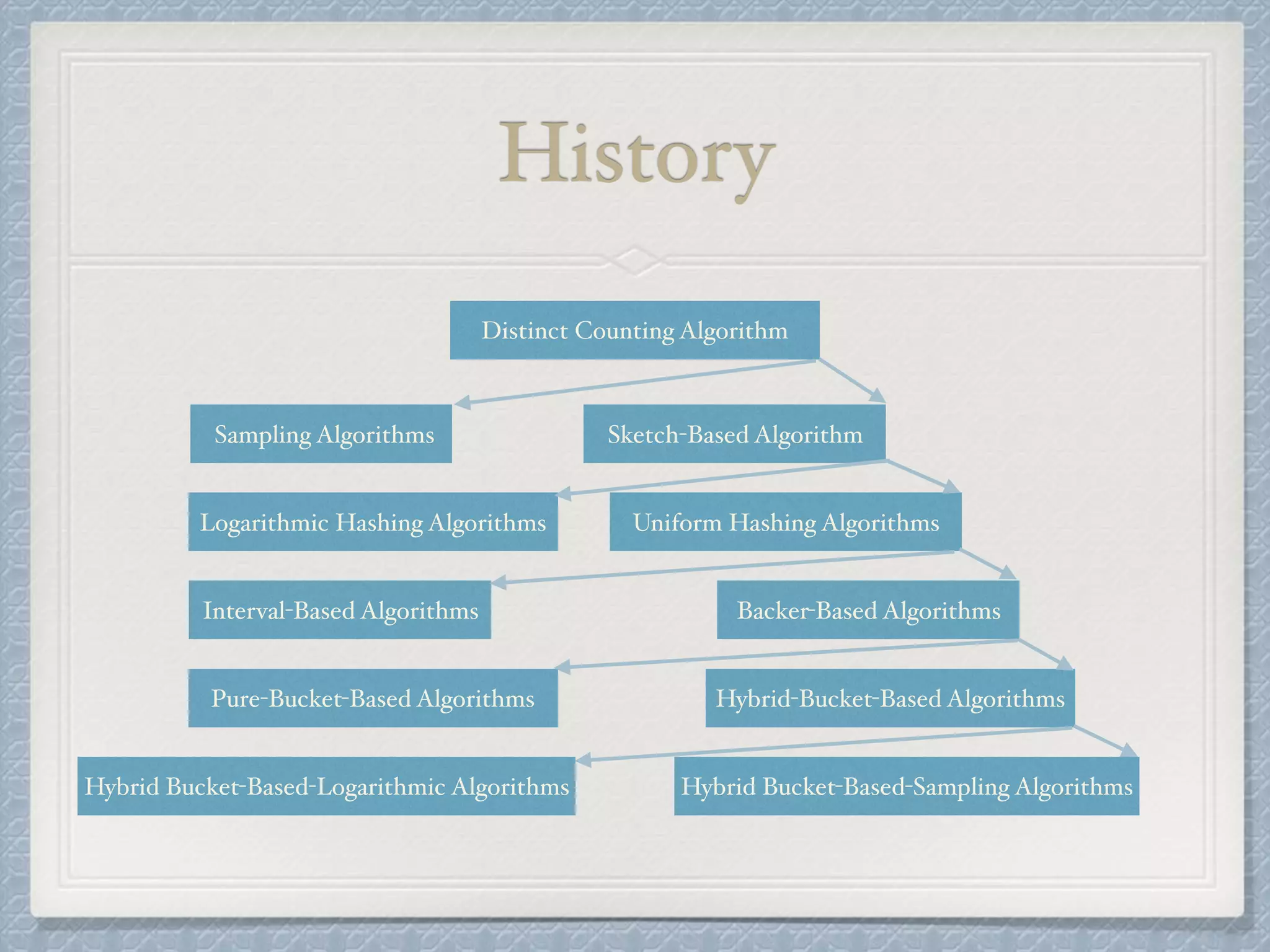
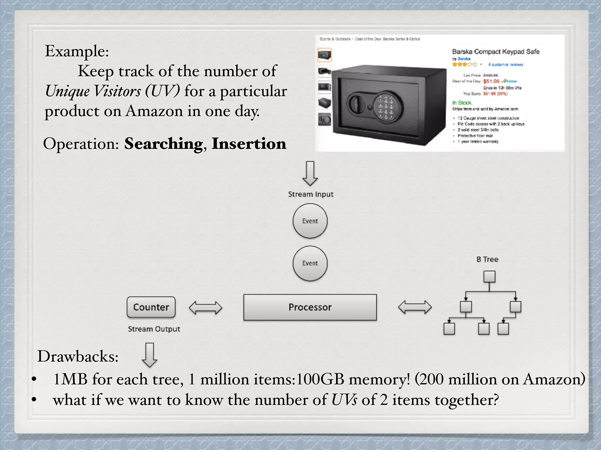
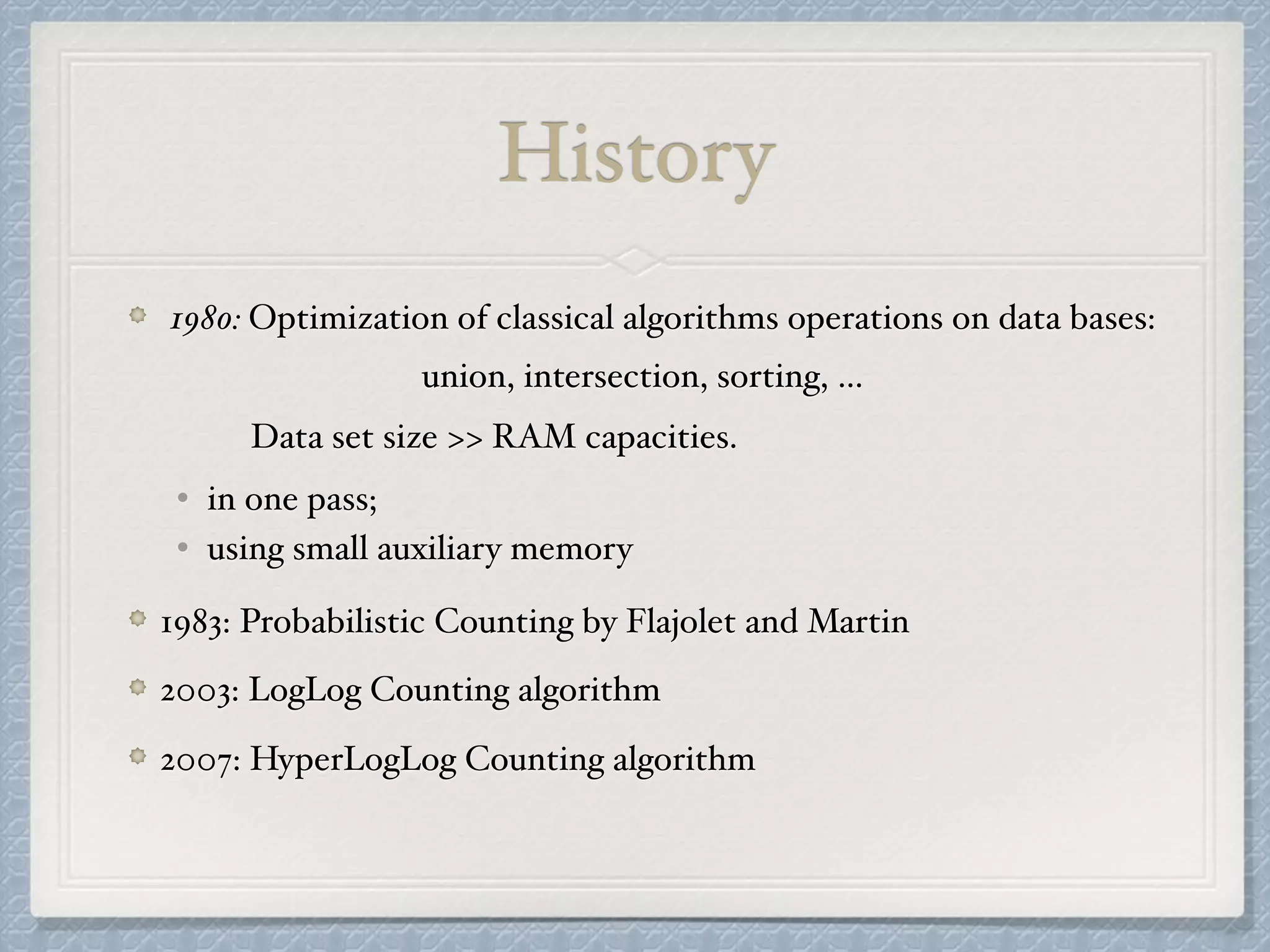
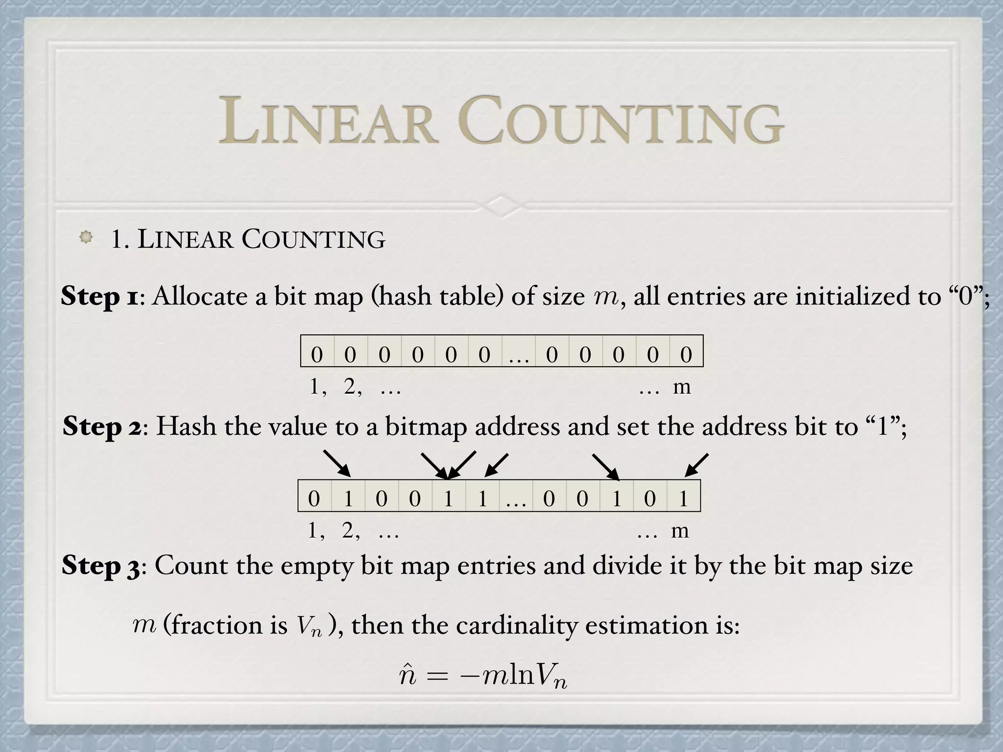
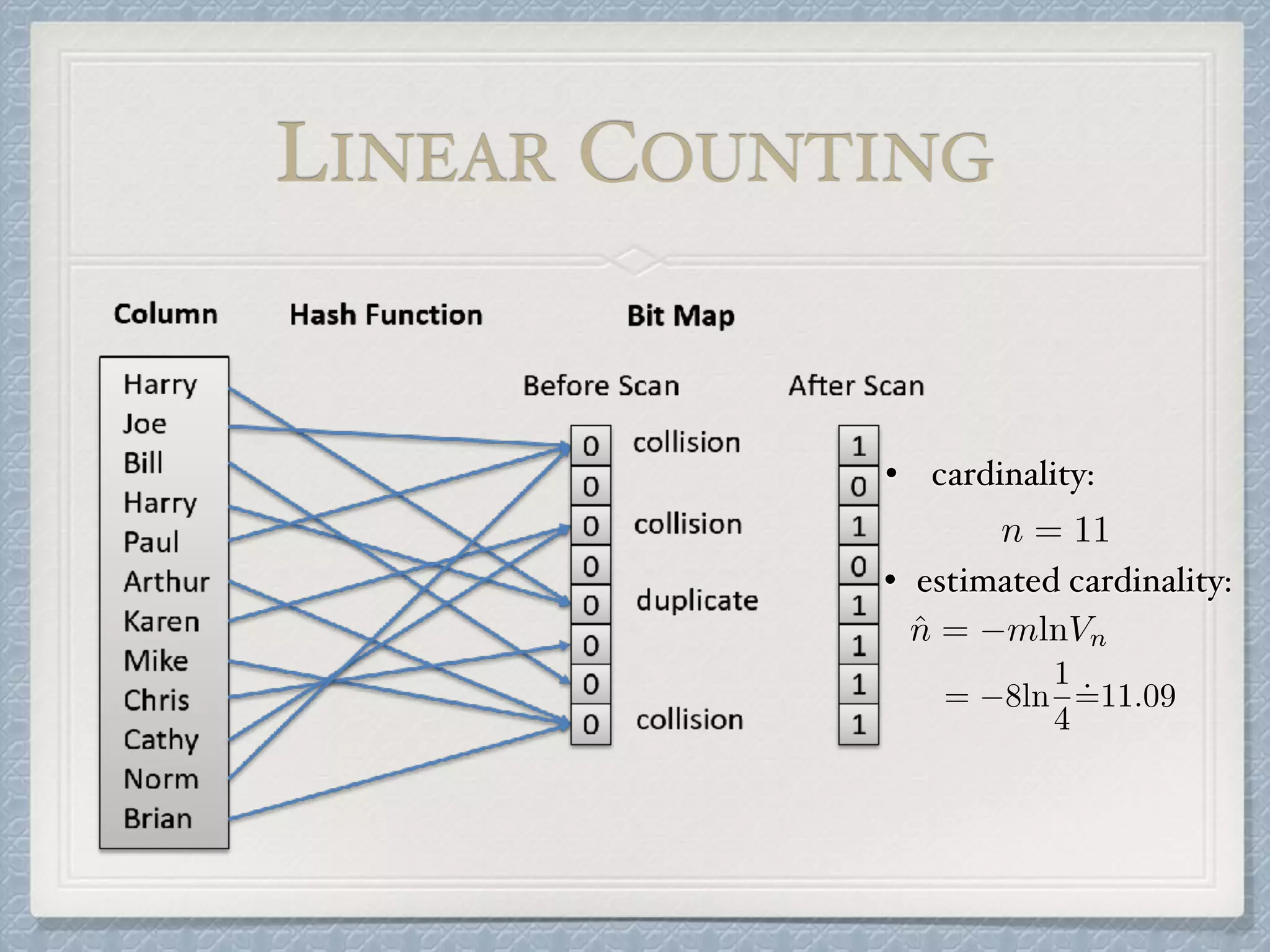
2. Questions
1. What is the cardinality of this data stream:
{1, 2, 4, 6, 8, 9, 2, 3, 11, 3, 1, 4}
2. Remember we use “bit pattern observables” to estimate
cardinality, describe the basic idea behind it.
3. How is the “buckets” useful in LOGLOG COUNTING algorithm?
n
4. Definition:
Instance: A stream of elements with repetitions, and
an integer . Let be the number of distinct elements, namely
, and let these elements be .
Overview
x1, x2, ..., xs
m n
n =| {x1, x2, ..., xs} || {e1, e2, ..., en} |
ˆn n
m ⌧ n
a, b, a, c, d, b, d
n =| {a, b, c, d} |= 4
mObjective: Find an estimate of using only storage units, where
.
e.g. Count the cardinality of the stream: . For this
instance, .
5. Example:
Keep track of the number of
Unique Visitors (UV) for a particular
product on Amazon in one day.
• 1MB for each tree, 1 million items:100GB memory! (200 million on Amazon)
• what if we want to know the number of UVs of 2 items together?
Drawbacks:
Operation: Searching, Insertion
6. Other Applications
Application:
Networking / Traffic monitoring
• Detection of worm propagation
• Network attacks
• Link-based spam
Data mining of massive data set
• Natural language texts
• Biological data
• Large structured databases
Google: Sawzall, Dremel and PowerDrill
7. 1980: Optimization of classical algorithms operations on data bases:
union, intersection, sorting, …
Data set size >> RAM capacities.
• in one pass;
• using small auxiliary memory
1983: Probabilistic Counting by Flajolet and Martin
2003: LogLog Counting algorithm
2007: HyperLogLog Counting algorithm
History
8. 1. LINEAR COUNTING
0 0 0 0 0 0 … 0 0 0 0 0
1, 2, … … m
LINEAR COUNTING
0 1 0 0 1 1 … 0 0 1 0 1
1, 2, … … m
Step 2: Hash the value to a bitmap address and set the address bit to “1”;
m Vn
ˆn = mlnVn
Step 3: Count the empty bit map entries and divide it by the bit map size
(fraction is ), then the cardinality estimation is:
mStep 1: Allocate a bit map (hash table) of size , all entries are initialized to “0”;
9. n = 11
• cardinality:
• estimated cardinality:
ˆn = mlnVn
= 8ln
1
4
˙=11.09
LINEAR COUNTING
10. Let stands for the event that
box is empty:
Let denote the number of
empty boxes:
P(Aj) =
✓
1
1
m
◆n
Aj
P(Aj Ak) =
✓
1
2
m
◆n
, j 6= k
Un
E(Un) =
mX
j=1
P(Aj) = m
✓
1
1
m
◆n
⇠= me n/m
ˆn = mln
E(Un)
m
balls
boxes
n
m
j
LINEAR COUNTING
11. Algorithm Basic Linear Counting:
let = the key for the th tuple in the relation.
initialize the bit map to “0”s.
for =1 to do
hash_value = hash( )
bit map(hash_value)=“1”
end for
= number of “0”s in the bit map
= /m
keyi i
i q
keyi
Un
Vn Un
ˆn = mlnVn
LINEAR COUNTING
12. How to choose size ? The mean number of empty boxes must be
a standard deviations from zero:
Lemma: The limiting distribution of , the number of empty
boxes, is Poisson with the expected value of
as
Thus,
The fill-up probability is then obtained as
If , that is , ,
m
E(Un) a ⇥ StdDev(Un) > 0
Un
me n/m
! n, m ! 1
lim
n,m!1
Pr(Un = k) = ( k
/k!)e
Pr(Un = 0) = e
a > 5 E(Un) >
p
5 · StdDev(Un) >
p
5
Constraint 1:
Pr(Un = 0) < e 5
˙=0.007(0.7%)
13. Suppose the user what to limit the standard error to , we have
or equivalently as
✏
((et
t 1)/m)1/2
t
< ✏
m >
et
t 1
(✏t)2
Constraint 2:
15. “01001101001…”
for each string , let denote the position of its first 1-
bit:
and denote the data set after hashing. Clearly, we can expect about
amongst the distinct elements of to have a -value equal to
, so
is a rough indication on the value of .
x 2 {0, 1}1
⇢(x)
⇢(1...) = 1, p(001) = 3, etc
n/2k
M
M ⇢
k
R(M) := max
1jn
⇢(x)
log2n
LOGLOG COUNTING
Basic Idea: (Bit pattern observables)
Hash the each data to binary strings like
16. LOGLOG COUNTING
0 0 1 0 1 1 0 1 0 0 1 1 1 0 1 0 0 1 0 0 0 1 0 1
the hash function hash each value to a binary string, suppose, “90001” to:
the first 1 bit of this {0,1}-string is 3, .⇢(001011...) = 3
Suppose here comes a data stream: {234, 39102, 3, 4556, 90011, 87, …},
It has high variability: one experiment cannot suffice to obtain accurate
predictions.
Stochastic Averaging: emulating the effect of experiments.m
hash value
17. LOGLOG COUNTING
0 0 1 0 1 1 0 1 0 0 1 1 1 0 1 0 0 1 0 0 0 1 0 1
m
hash value
bucket index
Stochastic Averaging: emulating the effect of experiments.
Use the last 8 digits to represent bucket number:
8 bits can represent buckets (experiments).m = 28
= 256
http://content.research.neustar.biz/blog/hll.html
18. 2. LOGLOG COUNTING algorithm
LOGLOG COUNTING ( : multiset of hashed values; ):
initialize to “0”;
let be the rank of the first 1-bit from the left in :
for do
set (value of first k bits in base 2)
set
return as cardinality estimate.
M m ⌘ 2k
M(1)
, M(2)
, ..., M(m)
⇢(y) y
x = b1b2... 2 M
j := hb1, ..., bki
M(j)
:= max(M(j)
, ⇢(bk+1bk+2...))
E := ↵mm2
1
m
P
j M(j)
LOGLOG COUNTING
19. Theorem: Let be a function that tends to infinity arbitrarily slowly and
consider the function
Then, the -restricted algorithm and the LOGLOG algorithm provide the same
output with probability tending to 1 as tends to infinity.
e.g. Count cardinality till (a hundred million), adopt buckets;
each bucket is visited (roughly): times;
we have , adopt , each bucket: 5 bits;
Totally 1024*5/8=640 bytes! (with a standard error of 4%)
!(n)
l(n) = log2log2(
n
m
) + !(n)
l(n)
n
227
m = 1024 = 210
n/m = 217
log2log2217
˙=4.09 ! = 0.91
LOGLOG COUNTING
20. HYPERLOGLOG COUNTING
HYPERLOGLOG COUNTING
LOGLOG COUNTING algorithm with Harmonic Mean
E := ↵mm2
1
m
P
j M(j)
1
m
(M(1)
+ M(2)
+ · · · + M(m)
)
Arithmetic mean
m
1
2M(1) + 1
2M(2) + · · · + 1
2M(m)
E := ↵mm2
0
@
mX
j=1
2 M[j]
1
A
1
Harmonic Mean
21. 3. HYPERLOGLOG COUNTING algorithm
HYPERLOGLOG COUNTING( input : multiset of items):
assume with
initialize a collection of integers, to ;
for do
set (value of first k bits in base 2)
set (the binary address determined
by the first bits of )
set set
compute
return
m = 2b b 2 Z>0
m M[1], ..., M[m] 1
v 2 M
x := h(v)
j = 1 + hx1x2...xbi2
b x
w := xb+1xb+2...; M[j] := max(M[j], ⇢(!))
Z :=
0
@
mX
j=1
2 M[j]
1
A
1
E := ↵mm2
Z
HYPERLOGLOG COUNTING
M
32. if then
Let V be the number of registers equal to 0.
V ~=0 then set E := LinearCounting(m, V )
else
do nothing
end
if then
E := E
if
end
return E
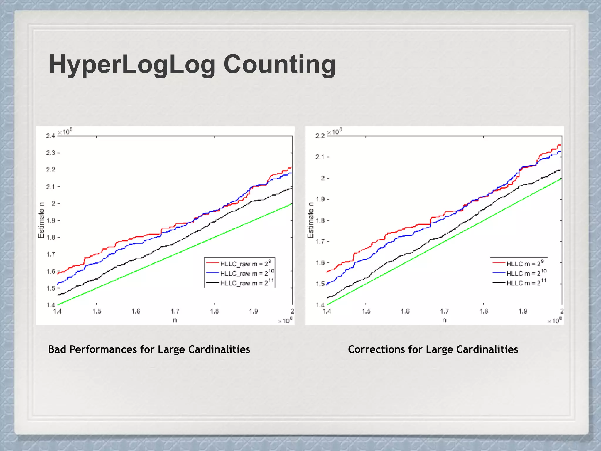
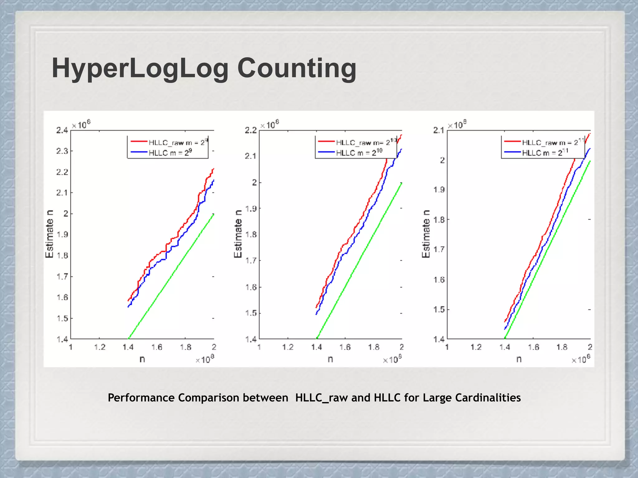
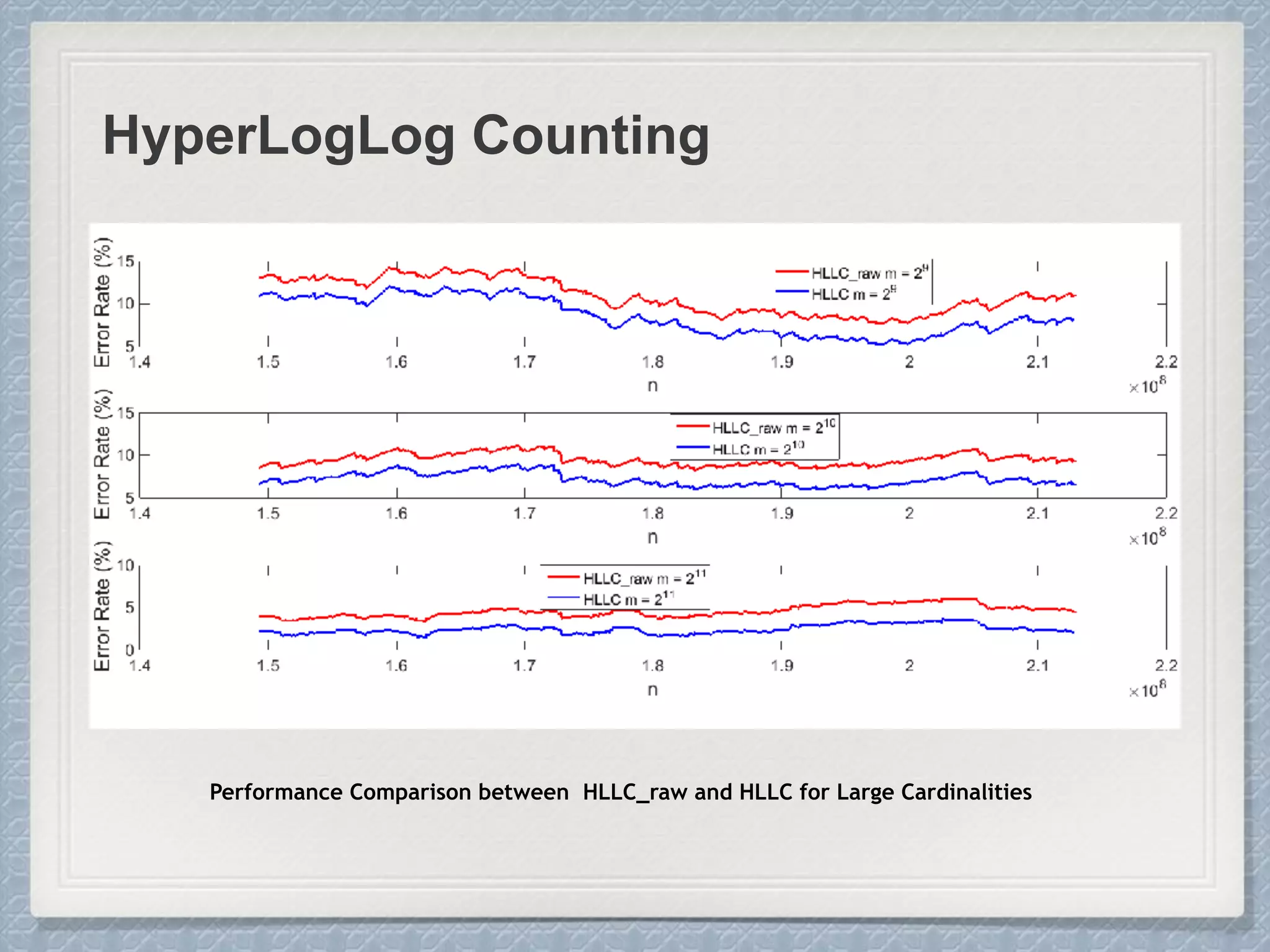
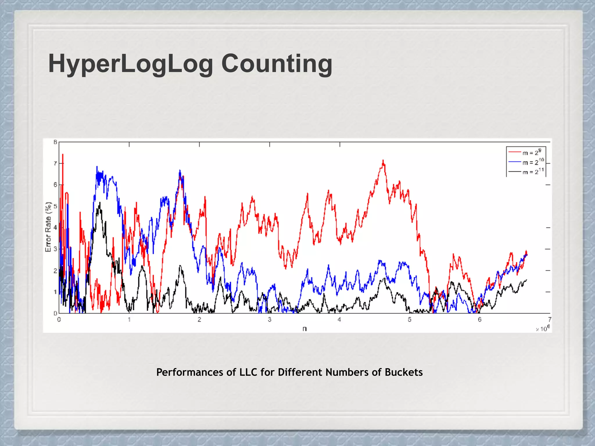
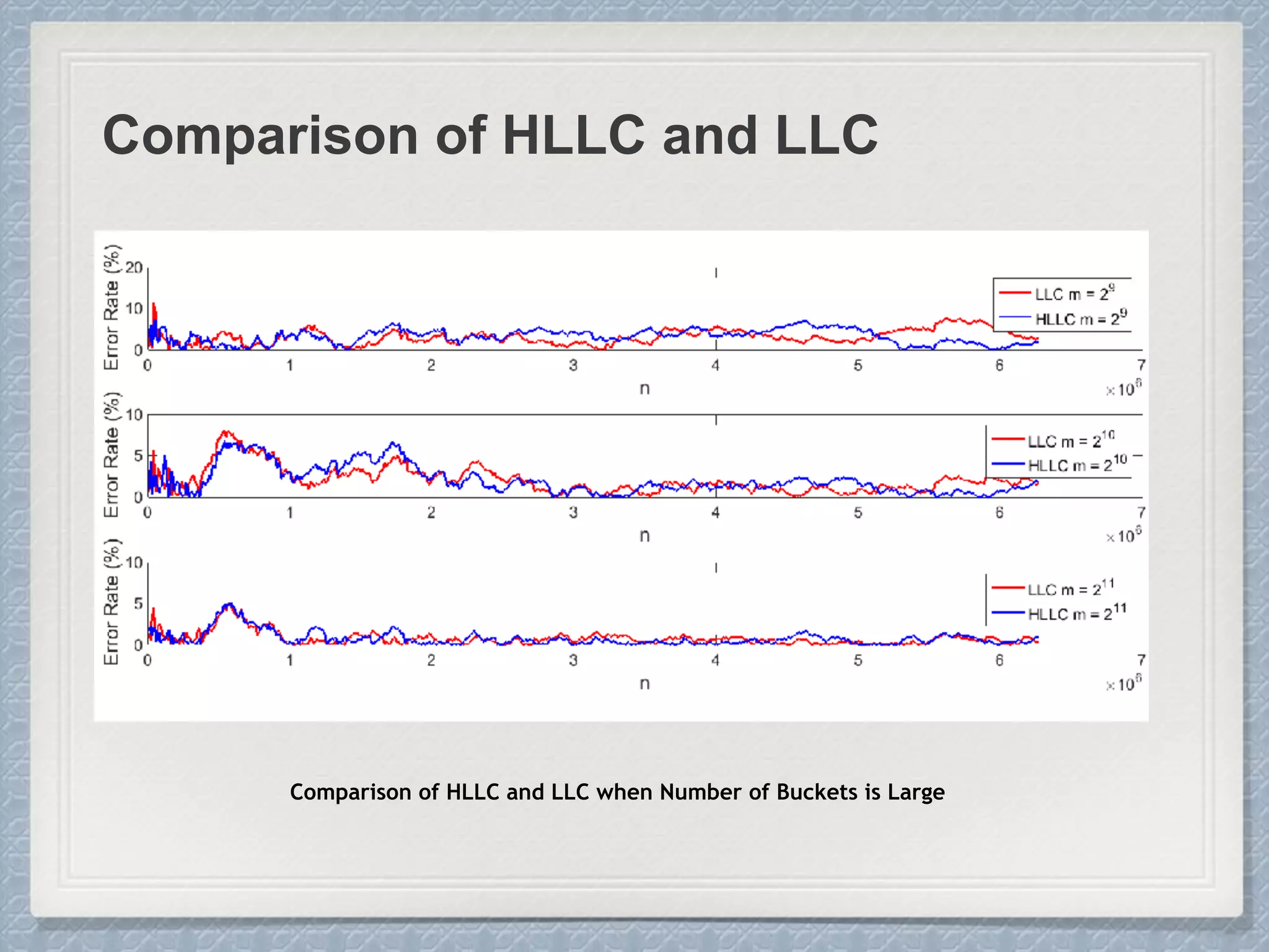
Large Cardinalities:
A hash function of L bits can at most
distinguish 2L different values, and as the
cardinality n approaches 2L, hash
collisions become more and more likely
and accurate estimation gets impossible.
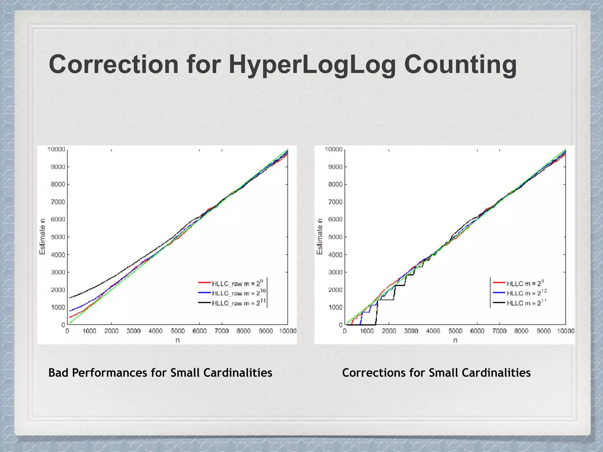
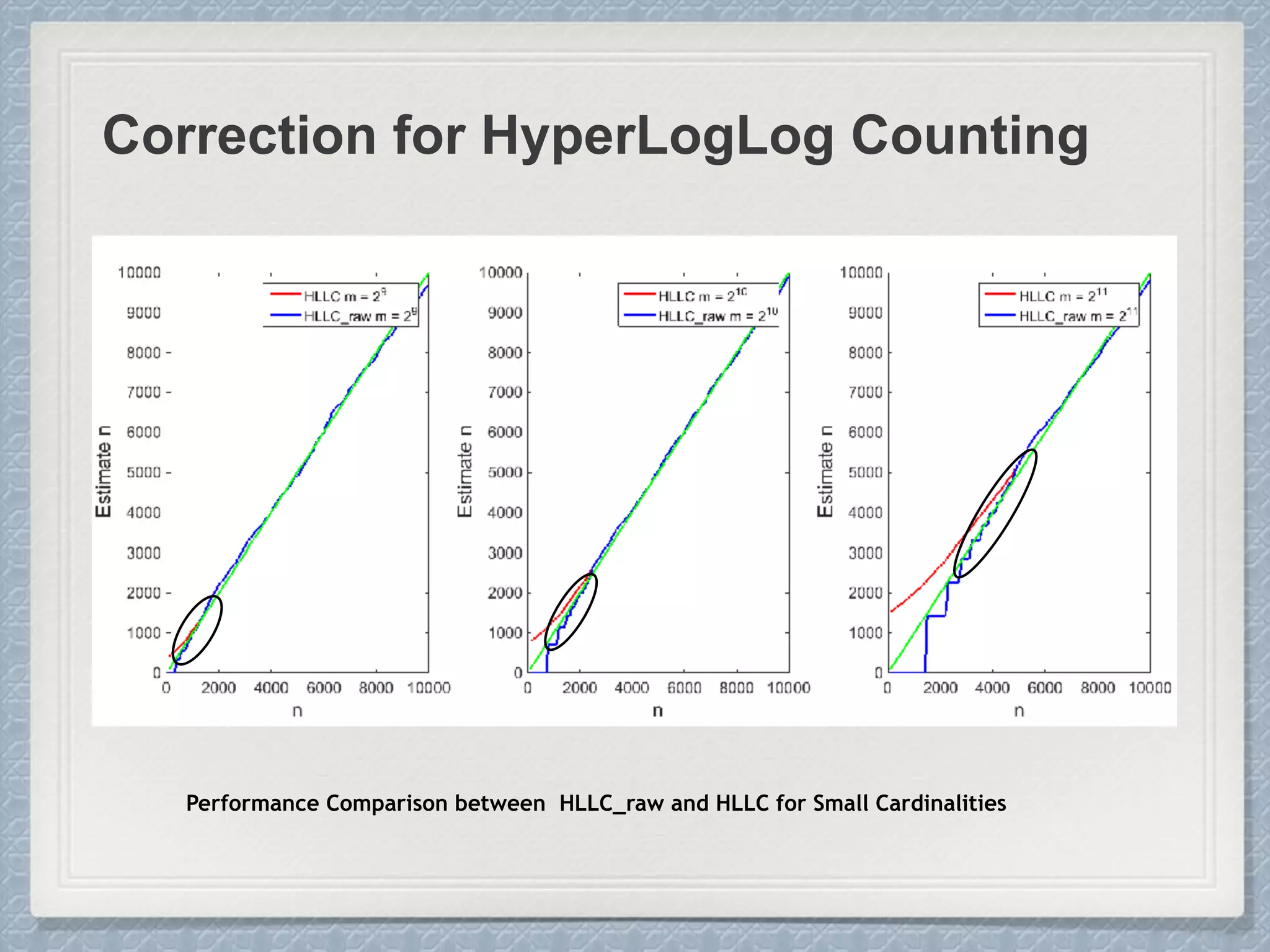
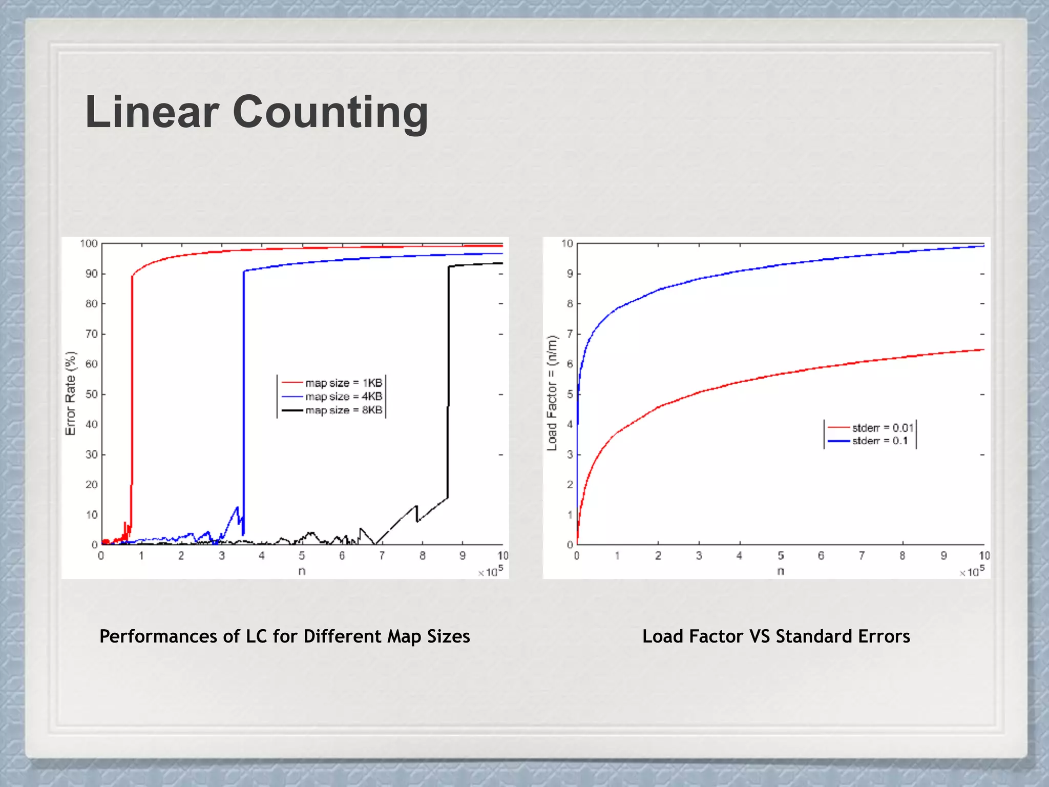
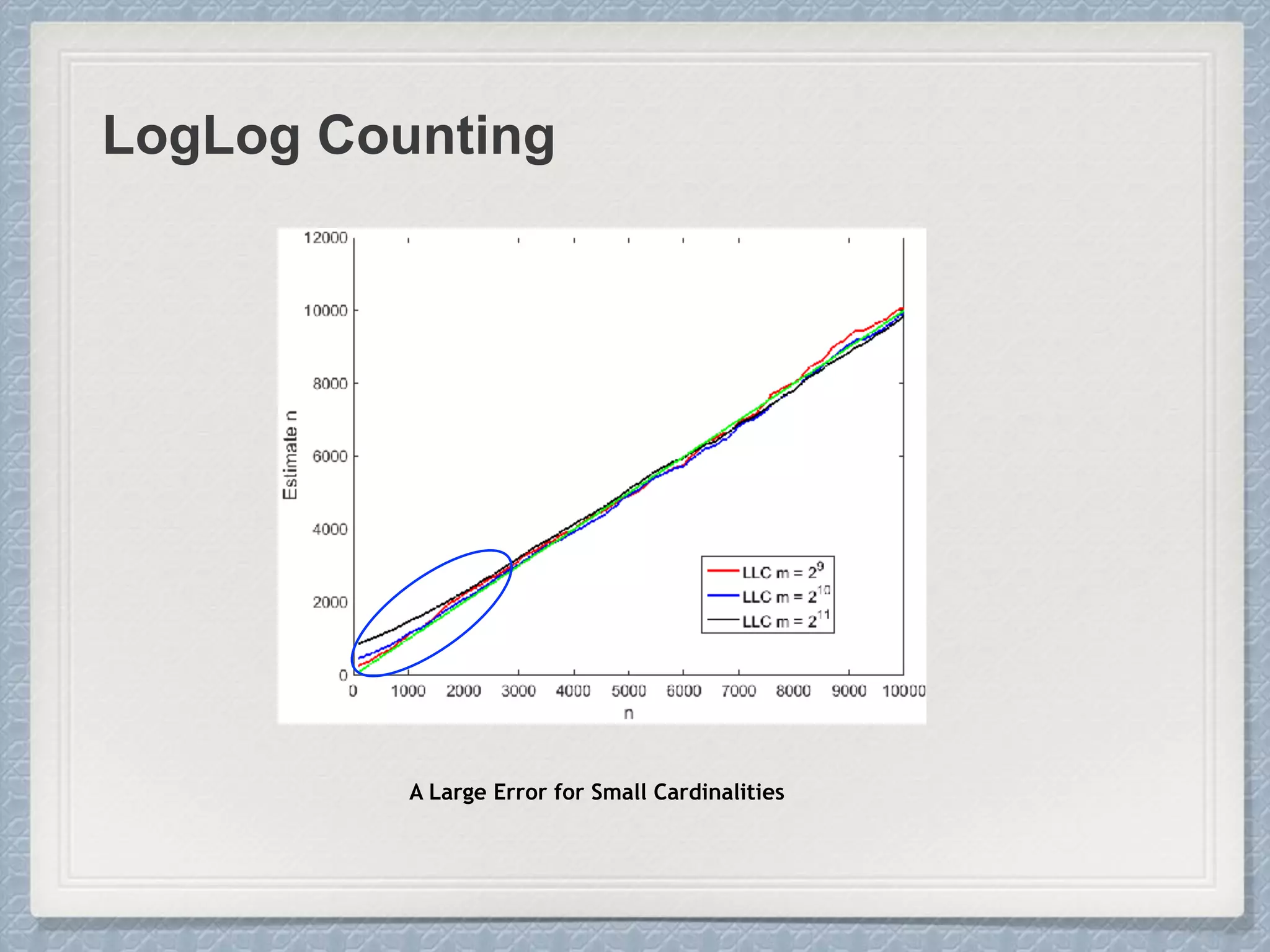
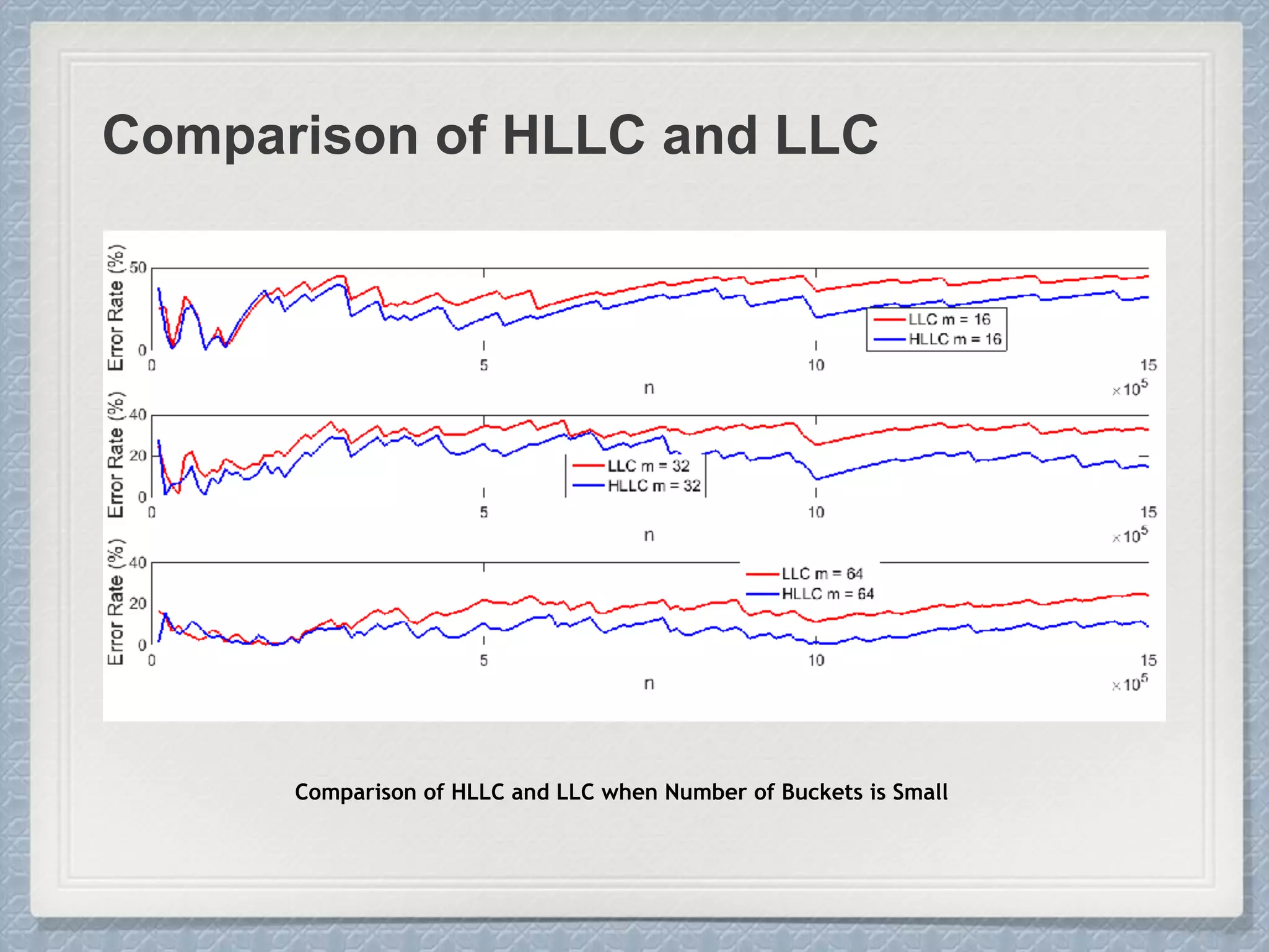
Small Cardinalities:
When cardinality is small, the
proportion of un-hit bucket is large,
which leads to inaccurate estimation.
E := ↵mm2
0
@
mX
j=1
2 M[j]
1
A
2
E <=
5
2
m
E
1
30
232
E = 232
log(1 E/232
)
E
1
30
232
The “raw” estimate:
33. Correction for HyperLogLog Counting
Bad Performances for Small Cardinalities Corrections for Small Cardinalities
34. Correction for HyperLogLog Counting
Performance Comparison between HLLC_raw and HLLC for Small Cardinalities
39. Reference
Whang, Kyu-Young, Brad T. Vander-Zanden, and Howard M. Taylor. "A linear-time
probabilistic counting algorithm for database applications." ACM Transactions on
Database Systems (TODS) 15.2 (1990): 208-229.
Durand, Marianne, and Philippe Flajolet. "Loglog counting of large cardinalities."
Algorithms-ESA 2003. Springer Berlin Heidelberg, 2003. 605-617.
Flajolet, Philippe, et al. "Hyperloglog: the analysis of a near-optimal cardinality estimation
algorithm." DMTCS Proceedings 1 (2008).
Heule, Stefan, Marc Nunkesser, and Alexander Hall. "HyperLogLog in practice: algorithmic
engineering of a state of the art cardinality estimation algorithm." Proceedings of the 16th
International Conference on Extending Database Technology. ACM, 2013.
Metwally, Ahmed, Divyakant Agrawal, and Amr El Abbadi. "Why go logarithmic if we can go
linear?: Towards effective distinct counting of search traffic." Proceedings of the 11th
international conference on Extending database technology: Advances in database
technology. ACM, 2008.