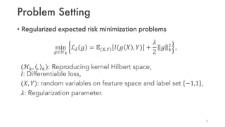
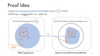
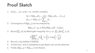
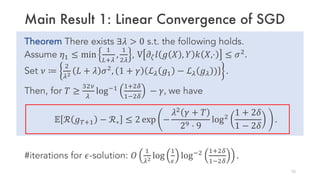
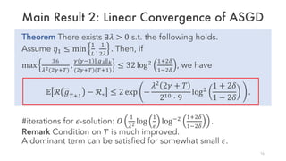
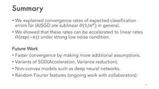
Stochastic Gradient Descent with Exponential Convergence Rates of Expected Classification Errors The document presents two main results: 1) Stochastic Gradient Descent (SGD) achieves linear convergence rates for expected classification error under a strong low noise condition. The number of iterations needed for an epsilon solution is O(log(1/epsilon)). 2) Averaged SGD (ASGD) achieves even faster linear convergence rates under the same condition, requiring O(log(1/epsilon)) iterations for an epsilon solution. 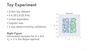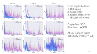The results improve upon prior work by showing faster-than-sublinear convergence rates for more suitable loss functions like logistic loss. Toy experiments demonstrate the theoretical findings.

1. Stochastic Gradient Descent with
Exponential Convergence Rates of
Expected Classification Errors
Atsushi Nitanda and Taiji Suzuki
AISTATS
April 18th, 2019
Naha, Okinawa
RIKEN AIP
1, 2 1, 2
1 2

2. Overview
• Topic
Convergence analysis of (averaged) SGD for binary classification
problems.
• Key assumption
Strongest version of low noise condition (margin condition) on the
conditional label probability.
• Result
Exponential convergence rates of expected classification errors
2

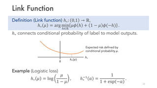
3. Background
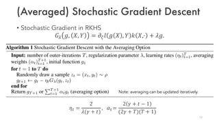
• Stochastic Gradient Descent (SGD)
Simple and effective method for training machine learning models.
Significantly faster than vanilla gradient descent.
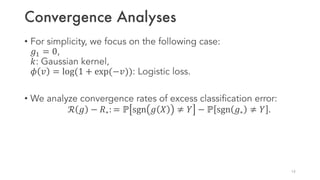
• Convergence Rates
Expected risk: sublinear convergence 𝑂(1/𝑛&
), (𝛼 ∈ [1/2,1]).
Expected classification error: How fast dose it converge?
GD SGD
SGD: 𝑔/01 ← 𝑔/ − 𝜂𝐺6(𝑔/, 𝑍/) (𝑍/ ∼ 𝜌),
GD : 𝑔/01 ← 𝑔/ − 𝜂𝔼;<∼= 𝐺6 𝑔/, 𝑍/
Cost per iteration:
1 (SGD) vs #data examples (GD)
3

4. Background
Common way to bound classification error.
• Classification error bound via consistency of loss functions：
[T. Zhang(2004), P. Bartlett+(2006)]
ℙ sgn 𝑔 𝑋 ≠ 𝑌 − ℙ sgn 2𝜌 1 𝑋 − 1 ≠ 𝑌 ≲ ℒ 𝑔 − ℒ∗
H
,
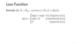
𝑔: predictor, ℒ∗: Bayes optimal for ℒ,
𝜌 1 𝑋 : conditional probability of label 𝑌 = 1.
𝑝 = 1/2 for logistic, exponential, and squared losses.
• Sublinear convergence 𝑂
1
KLM of excess classification error.
4
Excess classification error Excess risk

5. Background
Faster convergence rates of excess classification error.
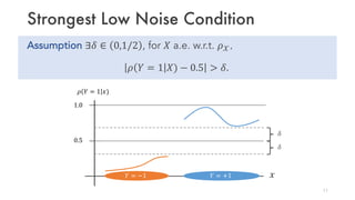
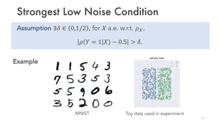
• Low noise condition on 𝜌 𝑌 = 1 𝑋)
[A.B. Tsybakov(2004), P. Bartlett+(2006)]
improves the consistency property,
resulting in faster rates: 𝑂
1
K
. (still sublinear convergence)
• Low noise condition (strongest version)
[V. Koltchinskii & O. Benzosova(2005), J-Y. Audibert & A.B. Tsybakov(2007)]
accelerates the rates for ERM to linear rates 𝑂 exp(−𝑛) .
5

6. Background
Faster convergence rates of excess classification error for SGD.
• Linear convergence rate
[L. Pillaud-Vivien, A. Rudi, & Francis Bach(2018)]
has been shown for the squared loss function under the strong low
noise condition.
• This work
shows the linear convergence for more suitable loss functions (e.g.,
logistic loss) under the strong low noise condition.
6

7. Outline
• Problem Settings and Assumptions
• (Averaged) Stochastic Gradient Descent
• Main Results: Linear Convergence Rates of SGD and ASGD
• Proof Idea
• Toy Experiment
7

8. Problem Setting
• Regularized expected risk minimization problems
min
S∈ℋU
ℒ6 𝑔 = 𝔼(V,W) 𝑙(𝑔 𝑋 , 𝑌) +
𝜆
2
𝑔 [
,
(ℋ[, , [): Reproducing kernel Hilbert space,
𝑙: Differentiable loss,
(𝑋, 𝑌): random variables on feature space and label set −1,1 ,
𝜆: Regularization parameter.
8

9. Loss Function
Example ∃𝜙: ℝ → ℝbc：convex s.t. 𝑙 𝜁, 𝑦 = 𝜙 𝑦𝜁 ,
𝜙 𝑣 = g
log(1 + exp −𝑣 ) 𝑙𝑜𝑔𝑖𝑠𝑡𝑖𝑐 𝑙𝑜𝑠𝑠 ,
exp −𝑣 𝑒𝑥𝑝𝑜𝑛𝑒𝑛𝑡𝑖𝑎𝑙 𝑙𝑜𝑠𝑠 ,
𝑣
𝑠𝑞𝑢𝑎𝑟𝑒𝑑 𝑙𝑜𝑠𝑠 .
9

10. Assumption
- sup
𝒳
𝑘(𝑥, 𝑥) ≤ 𝑅
,
- ∃𝑀 > 0, 𝜕• 𝑙 𝜁, 𝑦 ≤ 𝑀,
- ∃𝐿 > 0 ∀𝑔, ℎ ∈ ℋ[, ℒ 𝑔 + ℎ − ℒ 𝑔 − ∇ℒ(𝑔), ℎ [ ≤
†
ℎ [
,
- 𝜌 𝑌 = 1 𝑋 ∈ 0,1 , 𝑎. 𝑒.,
- ℎ∗ : increasing function on 0,1 ,
- sgn 𝜇 − 0.5 = sgn ℎ∗ 𝜇 ,
- 𝑔∗ ≔ arg min
S:Œ•Ž••‘Ž’“•
ℒ 𝑔 ∈ ℋ[.
Remark Logistic loss satisfies these assumptions.
The other loss functions also satisfy them by restricting Hypothesis space.
10
Link function:
ℎ∗ 𝜇 = arg min
”∈ℝ
𝜇𝜙 ℎ + 1 − 𝜇 𝜙(−ℎ) .

11. Strongest Low Noise Condition
Assumption ∃𝛿 ∈ 0,1/2 , for 𝑋 a.e. w.r.t. 𝜌 𝒳，
𝜌 𝑌 = 1 𝑋) − 0.5 > 𝛿.
11
𝜌 𝑌 = 1 𝑥)
𝒳
0.5
1.0
𝑌 = −1 𝑌 = +1
𝛿
𝛿

12. Strongest Low Noise Condition
Assumption ∃𝛿 ∈ 0,1/2 , for 𝑋 a.e. w.r.t. 𝜌 𝒳，
𝜌 𝑌 = 1 𝑋) − 0.5 > 𝛿.
MNIST
12
Toy data used in experiment
Example

13. (Averaged) Stochastic Gradient Descent
13
• Stochastic Gradient in RKHS
𝐺6 𝑔, 𝑋, 𝑌 = 𝜕• 𝑙 𝑔 𝑋 , 𝑌 𝑘 𝑋,⋅ + 𝜆𝑔.
𝜂/ =
2
𝜆(𝛾 + 𝑡)
, 𝛼/ =
2 𝛾 + 𝑡 − 1
(2𝛾 + 𝑇)(𝑇 + 1)
Note: averaging can be updated iteratively.

14. Convergence Analyses
• For simplicity, we focus on the following case:
𝑔1 = 0,
𝑘: Gaussian kernel,
𝜙 𝑣 = log(1 + exp(−𝑣)): Logistic loss.
• We analyze convergence rates of excess classification error:
ℛ 𝑔 − 𝑅∗: = ℙ sgn 𝑔 𝑋 ≠ 𝑌 − ℙ sgn 𝑔∗ ≠ 𝑌 .
14

15. Main Result 1: Linear Convergence of SGD
Theorem There exists ∃𝜆 > 0 s.t. the following holds.
Assume 𝜂1 ≤ min
1
†06
,
1
6
, V 𝜕• 𝑙 𝑔 𝑋 , 𝑌 𝑘 𝑋,⋅ ≤ 𝜎
.
Set 𝜈 ≔
6• 𝐿 + 𝜆 𝜎
, 1 + 𝛾 ℒ6 𝑔1 − ℒ6 𝑔6 ) .
Then, for 𝑇 ≥
Ÿ
6
log¡1 10¢
1¡¢
− 𝛾, we have
𝔼 ℛ 𝑔£01 − ℛ∗ ≤ 2 exp −
𝜆
𝛾 + 𝑇
2¤ ⋅ 9
log
1 + 2𝛿
1 − 2𝛿
.
#iterations for 𝜖-solution: 𝑂
1
6• log
1
§
log¡ 10¢
1¡¢
.
15

16. Main Result 2: Linear Convergence of ASGD
Theorem There exists ∃𝜆 > 0 s.t. the following holds.
Assume 𝜂1 ≤ min
1
†
,
1
6
. Then, if
max
٬
6•(©0£)
,
© ©¡1 Sª U
(©0£)(£01)
≤ 32 log 10¢
1¡¢
, we have
𝔼 ℛ 𝑔£01
− ℛ∗ ≤ 2 exp −
𝜆
2𝛾 + 𝑇
21c ⋅ 9
log
1 + 2𝛿
1 − 2𝛿
.
#iterations for 𝜖-solution: 𝑂
1
6• log
1
§
log¡ 10¢
1¡¢
.
Remark Condition on 𝑇 is much improved.
A dominant term can be satisfied for somewhat small 𝜖.
16

17. Toy Experiment
• 2-dim toy dataset．
• 𝛿 ∈ 0.1, 0.25, 0.4 ．
• Linear separable．
• Logistic loss．
• 𝜆 was determined by validation．
Right Figure
Generated samples for 𝛿 = 0.4.
𝑥1 = 1 is the Bayes optimal.
17

18. 18
From top to bottom:
1. Risk value
2. Class. error
3. Excess class. error
/Excess risk value
Purple line: SGD
Blue line : ASGD
ASGD is much faster
especially when 𝛿 = 0.4.

19. Summary
• We explained convergence rates of expected classification
errors for (A)SGD are sublinear 𝑂(1/𝑛&
) in general.
• We showed that these rates can be accelerated to linear rates
𝑂(exp(−𝑛)) under strong low noise condition.
Future Work
• Faster convergence by making more additional assumptions.
• Variants of SGD(Acceleration, Variance reduction).
• Non-convex models such as deep neural networks.
• Random Fourier features (ongoing work with collaborators).
19

20. References
- T. Zhang. Statistical behavior and consistency of classification methods based on convex risk
minimization. The Annals of Statistics, 2004.
- P. Bartlett, M. Jordan, & J. McAuliffe. Convexity, classification, and risk bounds. Journal of the
American Statistical Association, 2006.
- A.B. Tsybakov. Optimal aggregation of classifiers in statistical learning. The Annals of Statistics, 2004.
- V. Koltchinskii & O. Benzosova. Exponential convergence rates in classification. In International
Conference on Computational Learning Theory, 2005.
- J-Y. Audibert & A.B. Tsybakov. Fast learning rates for plug-in classifiers. The Annals of statistics, 2007.
- L. Bottou & O. Bousquet. The Tradeoffs of Large Scale Learning, Advances in Neural Information
Processing Systems, 2008.
- L. Pillaud-Vivien, A. Rudi, & Francis Bach. Exponential convergence of testing error for stochastic
gradient methods. In International Conference on Computational Learning Theory, 2018.
20

21. Appendix
21

22. Link Function
Definition (Link function) ℎ∗: 0,1 → ℝ,
ℎ∗ 𝜇 = arg min
”∈ℝ
𝜇𝜙 ℎ + 1 − 𝜇 𝜙(−ℎ) .
ℎ∗ connects conditional probability of label to model outputs.
Example (Logistic loss)
ℎ∗ 𝜇 = log
𝜇
1 − 𝜇
, ℎ∗
¡1
𝑎 =
1
1 + exp −𝑎
.
22
0
ℎ∗
Expected risk defined by
conditional probability 𝜇.
ℎ∗(𝜇)

23. Proof Idea
Set 𝑚 𝛿 ≔ max ℎ∗ 0.5 + 𝛿 , ℎ∗ 0.5 − 𝛿 .
Example (logistic loss) 𝑚 𝛿 = log
10¢
1¡¢
.
Through ℎ∗, noise condition is converted to: 𝑔∗ 𝑋 ≥ 𝑚 𝛿 .
Set 𝑔6 ≔ arg min
S∈ℋU
ℒ6(𝑔).
When 𝜆 is sufficiently small, 𝑔6 is close to 𝑔∗. Moreover,
Proposition
There exists 𝜆 s.t. 𝑔 − 𝑔6 [ ≤
Œ ¢
®
→ ℛ 𝑔 = ℛ∗.
23

24. 24
Analyze the convergence speed and probability to get in in RKHS.
𝜌(1|𝑋)
Space of conditional probabilities
Small ball which provides Bayes rule.
𝑔∗
𝑔6
Small ball mapped into .
RKHS (predictor)
SGD
ℎ∗
Recall ℎ∗ 𝜇 = arg min
”∈ℝ
𝜇𝜙 ℎ + 1 − 𝜇 𝜙(−ℎ) .
Proof Idea

25. Proof Sketch
1. Let 𝑍1, … , 𝑍£~𝜌 be i.i.d., random variables,
𝐷/: = 𝔼 ¶𝑔£01|𝑍1, … , 𝑍/ − 𝔼 ¶𝑔£01|𝑍1, … , 𝑍/¡1 ,
¶𝑔£01 = 𝔼 ¶𝑔£01 + ·
/¸1
£
𝐷/ .
2. Convergence of 𝔼 ¶𝑔£01 can be analyzed by
𝔼 ¶𝑔£01 − 𝑔6 ≤ 𝔼 ℒ6 𝔼 ¶𝑔£01 − ℒ6 𝑔6 .
3. Bound ∑/¸1
£
𝐷/ by Martingale inequality: for 𝑐£ s.t. ∑/¸1
£
𝐷/ º
≤ 𝑐£
,
ℙ ·
/¸1
£
𝐷/
[
≥ 𝜖 ≤ 2 exp −
𝜖
𝑐£
.
4. Bound 𝑐£ by stability of A(SGD).
5. Combining 1 and 2, probability to get Bayes rule can be obtained.
6. Finally, 𝔼 ¶𝑔£01 = ℙ ¶𝑔£01 𝑖𝑠 𝑛𝑜𝑡 𝐵𝑎𝑦𝑒𝑠 .
25