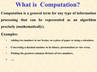
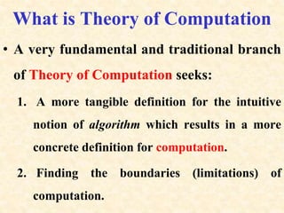
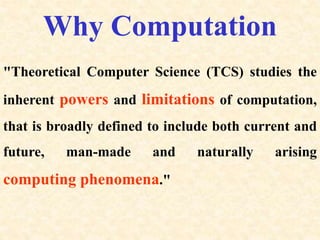
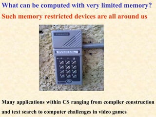
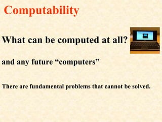
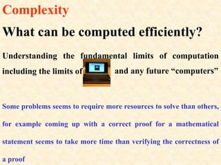
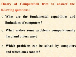
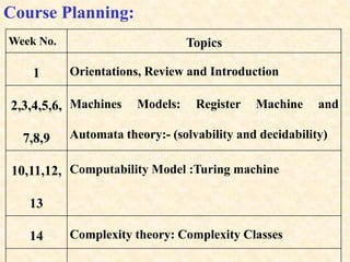
The document provides an overview of theory of computation. It defines computation as any type of information processing that can be represented as a precise algorithm. The theory of computation seeks to define algorithms formally and determine the capabilities and limitations of computation. It comprises three main areas: automata theory, computability, and complexity. Automata theory deals with solving simple decision problems. Computability determines which problems can be solved by computers. Complexity analyzes which problems can be computed efficiently. The document outlines a course on theory of computation covering these topics through examining machines, complexity classes, and the objectives of introducing different computation models and demonstrating uncomputable problems.

1. Theory of Computation
Mahmoud Ali Ahmed (PhD)
Dean
Faculty of Mathematical Sciences
U. of K.
email: mali@uofk.edu

2. What is Computation?
Computation is a general term for any type of information
processing that can be represented as an algorithm
precisely (mathematically).
Examples:
• Adding two numbers in our brains, on a piece of paper or using a calculator.
• Converting a decimal number to its binary presentation or vise versa.
• Finding the greatest common divisors of two numbers.
• …

3. What is Theory of Computation
• A very fundamental and traditional branch
of Theory of Computation seeks:
1. A more tangible definition for the intuitive
notion of algorithm which results in a more
concrete definition for computation.
2. Finding the boundaries (limitations) of
computation.

4. "Theoretical Computer Science (TCS) studies the
inherent powers and limitations of computation,
that is broadly defined to include both current and
future, man-made and naturally arising
computing phenomena."
Why Computation

5. What can be computed with very limited memory?
Such memory restricted devices are all around us
Many applications within CS ranging from compiler construction
and text search to computer challenges in video games

6. Computability
What can be computed at all?
and any future “computers”
There are fundamental problems that cannot be solved.

7. Complexity
What can be computed efficiently?
Understanding the fundamental limits of computation
including the limits of and any future “computers”
Some problems seems to require more resources to solve than others,
for example coming up with a correct proof for a mathematical
statement seems to take more time than verifying the correctness of
a proof

8. Theory of Computation tries to answer the
following questions :
o What are the fundamental capabilities and
limitations of computers?
o Which problems can be solved by computers
and which ones cannot?
o What makes some problems computationally
hard and others easy?

9. Based on this discussion, the course provides an
introduction to the theory of computation.
Traditionally, the study of theory of computation
comprises three central areas:
o Automata.
o Computability, and
o Complexity.

10. Objective of this Course
The aim of this course is to introduce several apparently different
formalizations of the informal notion of algorithm; to show that
they are equivalent; and to use them to demonstrate that there
are uncomputable functions and algorithmically undecidable
problems, and enables the student to be aware about:
• Automata theory (Dealing with solving simple decision
problems (solvable and unsolvable problems)),
• Computability (Computable problems: Turing machine), and
• Complexity (dealing with solvable problems: Time Complexity
(P and NP, and NP-complete) and Space Complexity (PSPACE,
NL)).

11. Course Outlines and Planning:
 Historical Perspective
 Review: Sets, Mathematical Notations, Graphs and Algorithms.
 Machines: Register Machine, Automat, Turing Machine
 Complexity Classes.
Course Outlines

12. Course Planning:
Week No. Topics
1 Orientations, Review and Introduction
2,3,4,5,6,
7,8,9
Machines Models: Register Machine and
Automata theory:- (solvability and decidability)
10,11,12,
13
Computability Model :Turing machine
14 Complexity theory: Complexity Classes

13. Student Evaluation
The student will be evaluated (Assessed) based on the
following:
 Course work
 Final exam
30%
70%

14. References
- Michael Sipser, Introduction to the Theory of Computation, PWS
Publishing Company, 1997.
- Mikhail J. Atallah and Mariana Blanton (Eds.), Algorithms and
Theory of Computation Handbook: General Concepts and Techniques,
CRC Press, New York, 2009 (2nd Edition).
Thomas Cormen, Charles Leiserson, Ronald Rivest, and Cliff Stein,
Introduction to Algorithms, McGraw Hill Publishing Company and
MIT Press, 2009 (3rd Edition).
Peter Linz, An Introduction to Formal Languages and Automata,
Jones and Bartlett Publishers, 2006.
- Other open sources (Internet)

15. Historical Perspectives
Euclid (350 B.C.) : Elements
Leonhard Euler (1707-1783) : Graph theory
Alan Turing (1912-1954) : Computability
Alonzo Church (1903-1995) : Lambda-calculus
John von Neumann (1903-1957) : Stored program
Claude Shannon (1916-2001) : Information theory
Noam Chomsky (1928-) : Formal languages
John Backus (1924-) : Functional programming
Edsger Dijkstra (1930-2002) : Structured programming
E N D

16. Review: Sets and Mathematical Notations
Definitions
SET:
It is an unordered collection of elements.
A= {1, 2, 3}
C={x|x is positive integer greater than or equal to x2}
B ={hi, there}
Example:
D = {3, 3.1, 3.14, 3.141, 3.1415, 3.14159, …}
A, B and C are finite sets while D is an infinite.

17. Set construction
| or means “such that”
Example:
E = {k | 0<k<4}
F = {k | k is a perfect square}
Set membership
means “belong to” or “ not belong to”,
7 {p | p prime}
q {0, 2, 4, 6,...}
Example:

18. Sets can contain other sets
Example:
G = {2, {5}}
H = {{{0}}} {0} 0 
S = {1, 2, 3, {1}, {{2}}}
Common Sets
Naturals: N = {1, 2, 3, 4, ...}
Integers: Z = {..,-2, -1, 0, 1, 2,..}
Rationals: Q = {a/b| a,b Z, b 0}
Reals: = {x | x a real #}

19. Empty set: Ø = {}
z+
= non-negative integers
= non-positive real


Multisets
E N D
a set with repeated elements allowed, (i.e., each
element has “multiplier”).
Example H = {0, 1, 2, 2, 2, 5, 5}

20. sequences
Definition: it an ordered list of elements
(0, 1, 2, 5) “4-tuple”
Example:
(1,2) “2-tuple”
Universal & Existential Quantification
“for all”
12
 xxxExample:

21. “there exists”
x| 2
 xxExample:
Combinations:
yxyx 
Boolean Operations
E N D
"" AND
"" OR
"" NOT
"" XOR
NAND
NOR

22. Logical Implication
"" implies
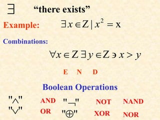
33
1 yxyx Example:
"" if and only if (iff)
"" equivalent
)]()[()( ABBABA 
or
ABBABA 

23. Example:
)(),max(),min( yxyxyx 
))()( PQQP 

24. Subsets
"" Subset notation
)( TxSxTS 
"" Proper Subset
))()(( TSTSTS 
))()(( TSSTTS 
SS  
SSS 

25. Union 
Example:
Example:
 TxSxxTS 
Intersection 
 TxSxxTS 

26. Set difference: S - T
Example:
 TxSxxTS 
Example:
TSTS 
 TxSxxTS 
Symmetric difference: S T

27. Universal set: U (everything)
Set Complement SorS
Disjoint sets:
Example
  SUSxxS 
Example:
TS
TSTS 
 SSSS

28. Set Identities
• Commutative Law:
Example
STTS 
STTS 
• Associative Law:
VTSVTS  )()(
VTSVTS  )()(
Example

29. Example:
• Associative Law:
)()()( VSTSVTS 
)()()( VSTSVTS 
Example:
• Absorption Law:
STSS  )(
STSS  )(

30. E N D
• DeMorgan's Laws:
Example
TSTS  )(
TSTS  )(

31. Proof Types
• Construction
• Contradiction
• Induction
• Counter-example

32. Graphs
Definition: Used to represent and model a problem
with special kind of relationship such as:
• Common relationships
• Communication networks
• Dependency constraints
• Reachability information
• + many more practical applications!

33. Definition:
Graph : is the combination of a set of
vertices , and a set of edges VVE V
),( EVG 
Pictorially: nodes & lines
Undirected Graphs
Definition: it the graph whose edges have no
direction.

34. a
b
c
e
d
V={a, b, c, d, e}
E={(c, a), (c, b), (c, d), (c, e), (a, b), (b, d), (d, e)}
Example

35. Directed Graphs
Definition: it the graph whose edges have direction.
Example
a
b
c e
d
V={a, b, c, d, e}
E={(a, b), (a, c), (b, c), (b, d), (d, c), (d, e), (c, e)}

36. Graph Terminology
Graph VVE ),,( EVG 
node vertex
edge arc
a
b
c e
d
f
For any pair of vertices (u, v) V are said to be
neighbors in G (u, v) or (v, u) is an edge of G.

a & b are neighbors. a & e are not neighbors.

37. Undirected Node Degree
Degree in undirected graphs:
Degree of any undirected node (vertex) of the
graphs is denoted by deg(v):
deg(v) = # of adjacent (incident) edges to vertex v in G
Example
deg(c)=4 deg(f)=0

38. directed Node Degree
Degree in directed graphs:
For any directed node (vertex) of the graph G
there are two types of degree.
In-deg(v): = # of incoming edges
Out-deg(v): = # of outgoing edges

39. Example
a
b
c
e
d
f
in-deg(c)=3 out-deg(c)=1
in-deg(f)=0 out-deg(f)=0

40. Complete Graph
Graph : is said to be complete if it
contains all edges, i. e.,   vuVVvuE  ,
),( EVKn 
a
b
c
e
d
f

41. Transition Graph
Definition: a transition graph is the
graph that can be defined by vertices
representing states (s) and directed lines
from each state (sk) to itself (loop) or to
another state (sj)
S1 S2

42. Graph Representation
a
b
c
d
Adjacency list:
1: (a) b d 
2: (a) c d 

43. Adjacency matrix:
a b c d
a 0 1 1 0
b 1 0 0 1
c 1 0 0 0
d 0 1 0 0

44. Algorithm
An algorithm is a set of unambiguous computational
procedures or steps that produce an output given an input.
Implementing an algorithm means transforming the set of
steps specified in the algorithm into a computer program.
Algorithms can be used to search, sort, and select data.
Data structures such as stacks, queues, arrays, and
trees can all have algorithms applied to them.

45. • The study and analysis of algorithms is
important as algorithms play a large role in
solving real world problems particularly in
business and other sectors where computing
has had a large impact.
Why it is important to study & analyze an algorithms?

46. • Different algorithms that accomplish the
same task can vary in their efficiency.
• This may not be important when used on a
small scale but when applied to large-scale
problems, efficiency becomes ever more
important.

47. • Algorithm analysis involves measuring how long
an algorithm will take to reach a result and
terminate.
What is an algorithm analysis?
• This may be measured by comparison with
other algorithms or it can be measured by
determining of what "order" the algorithm is.

48. Algorithm Complexity
Complexity is measured in the form of "Big-O"
notation. For example, "O(1)" means "order 1"
and describes programs where statements are
simply executed one after the other.
These programs/methods are described as
"constant time" methods .

49. Where loops are involved in the program,
this gives the program the order of "O(N)"
and these programs are known as having
"linear time".
Quadratic time methods involve loops being
nested within another loop and is given the
notation "O(N^2)".

50. By doubling the input of programs with
methods of complexity O(N^2), the number
of steps needed to execute the code to
completion will be multiplied by four.

51. Based on the complexity (the time needed to execute
the algorithm), algorithms can be classified into
several classes such as
• Linear Time Algorithms
• Exponential Time Algorithms
• Open Time (never complete) Algorithms

52. Running Time
Running time can be estimated in a more general
manner by using Pseudocode to represent the
algorithm as a set of fundamental operations which
can then be counted.
Pseudocode gives a high-level description of an
algorithm without the ambiguity associated with
plain text but also without the need to know the
syntax of a particular programming language.

53. Pseudocode contains all of the following
features:
Conventional loops:
If... then... else...
While... do...
Repeat... until...
For... do...

54. Method declaration:
Method name: Algorithm methodName(args)
Input description: Input...
Output description: Output...
Method calls:
var.methodName(args)
Return values: return...
Expressions:
Assignment: < --
Equality comparison: ==

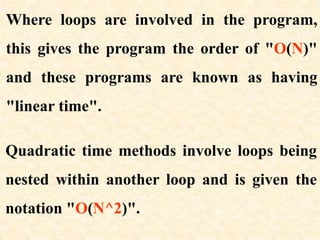
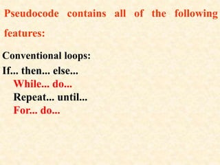
55. In a pseudo code description of an algorithm, each line
can be viewed as a certain number of operations which
can be counted and added up to find a total value (order
of algorithm) for the algorithm. Some examples are shown
below:
• varNumber <-- X[1]
(2 operations - 1 array value retrieval, 1 assignment).
• For a <-- 1 to n do...
(n operations - any operations within this loop will
then be multiplied by n also as they will be carried
out n times).
• return varNumber
(1 operations).