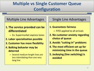
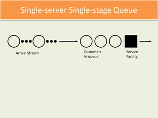
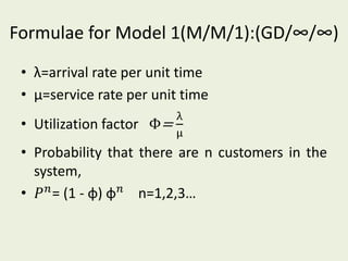
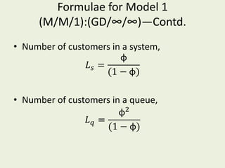
This document discusses queueing theory and queueing models. It defines key queue parameters like arrival and service processes, the number of servers, and queue discipline. Common distributions for these parameters are presented along with examples of single and multiple server, single and multiple stage queue configurations. Specific queueing models are introduced including the fundamental M/M/1 model. Finally, key performance measures and formulas are provided for analyzing the M/M/1 model like probability of n customers, average wait times, and more.

1. Queuing Theory
Y. B. Kumbhar
Ybk_aero@adcet.in

3. Structureof a queue

4. Queue Parameters
• Calling Population
• Arrival Process
• Queue Discipline
• Service Process
• Number of Servers

5. 5
1. The Calling Population
• Population of customers or jobs
• The size can be finite or infinite
– The latter is most common
• Can be homogeneous
– Only one type of customers/ jobs
• Or heterogeneous
– Several different kinds of customers/jobs

6. 6
2. Arrival Process
• In what pattern do jobs / customers arrive to
the queueing system?
– Distribution of arrival times?
– Batch arrivals?
– Finite population?
– Finite queue length?
• Poisson arrival process often assumed
– Many real-world arrival processes can be modeled
using a Poisson process

7. 7
3. Service Process
• How long does it take to service a job or
customer?
– Distribution of arrival times?
– Rework or repair?
– Service center (machine) breakdown?
• Exponential service times often assumed
– Works well for maintenance or unscheduled
service situations

8. 8
4. Number of Servers
• How many servers are available?
Single Server Queue
Multiple Server Queue

9. 9
Example – Two Queue Configurations
Servers
Multiple Queues
Servers
Single Queue

10. 10
1.The service provided can be
differentiated
– Ex. Supermarket express lanes
2. Labor specialization possible
3. Customer has more flexibility
4. Balking behavior may be
deterred
– Several medium-length lines are
less intimidating than one very
long line
1. Guarantees fairness
– FIFO applied to all arrivals
2. No customer anxiety regarding
choice of queue
3. Avoids “cutting in” problems
4. The most efficient set up for
minimizing time in the queue
5. Jockeying (line switching) is
avoided
Multiple vs Single Customer Queue
Configuration
Multiple Line Advantages Single Line Advantages

11. 11
5. Queue Discipline
• How are jobs / customers selected from the
queue for service?
– First Come First Served (FCFS)
– Shortest Processing Time (SPT)
– Earliest Due Date (EDD)
– Priority (jobs are in different priority classes)
• FCFS default assumption for most models

12. Single-server Single-stage Queue
Service
Facility
Customers
In queue
Arrival Stream

13. Multiple-server Single-stage Queue
Service
Facilities
Customers
In queue

14. Single-server Multiple-stage Queue
Service
Facility
Customers
In queue
Pharmacy Conveyor System >>>>>

15. Multiple-server Multiple-Stage Queue
Service
Facilities
Customers
In queue

16. Queuing Models
(P/Q /R):(X/Y/Z)
P : arrival rate distribution
Q : Service rate distribution
R : Number of servers
X : Service Discipline
Y : Max. customer permitted in system
Z : Size of calling population

17. Model 1: (M/M/1):(GD/∞/∞)
• M: Poisson arrival rate
• M: Poisson service rate
• 1: 1 Service server
• GD : General Discipline
• ∞ : Infinite customers are allowed in the
system
• ∞ : Customers are called from an infinite
polulation

18. Other models
• Model 2: ( M / M / C) : ( G D / ∞ / ∞ ) - C number of servers
• Model 3: ( M / M / 1 ) : ( G D / N/ ∞ ) - N customer allowed in
system
• Model 4: ( M / M / C) : ( G D / N/ ∞ )
• Model 5: ( M / M / 1 ) : ( G D / N/ N) - calling population is
finite (N)
• Model 6: ( M / M / C) : ( G D / N/ N)

19. Formulae for Model 1(M/M/1):(GD/∞/∞)
• λ=arrival rate per unit time
• μ=service rate per unit time
• Utilization factor Φ=
λ
μ
• Probability that there are n customers in the
system,
• 𝑃 𝑛
= (1 - φ) φ 𝑛
n=1,2,3…

20. Formulae for Model 1
(M/M/1):(GD/∞/∞)—Contd.
• Number of customers in a system,
𝐿 𝑠 =
φ
(1 − φ)
• Number of customers in a queue,
𝐿 𝑞 =
φ2
(1 − φ)

21. Formulae for Model 1
(M/M/1):(GD/∞/∞)—Contd.
• Average Waiting time of customers in a
system,
𝑊𝑠 =
1
(μ − λ)
• Average Waiting time of customers in a queue,
𝑊𝑞 =
φ
(μ − λ)