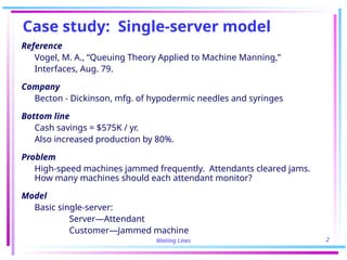
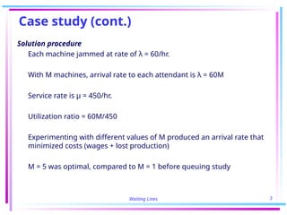
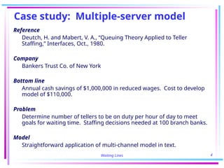
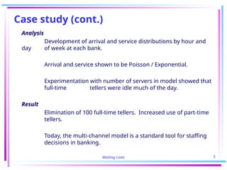
Service Operations
Service Operations
and
and
Waiting Lines
Waiting Lines
Waiting Lines 2
Case study: Single-server model
Reference
Vogel, M. A., “Queuing Theory Applied to Machine Manning,”
Interfaces, Aug. 79.
Company
Becton - Dickinson, mfg. of hypodermic needles and syringes
Bottom line
Cash savings = $575K / yr.
Also increased production by 80%.
Problem
High-speed machines jammed frequently. Attendants cleared jams.
How many machines should each attendant monitor?
Model
Basic single-server:
Server—Attendant
Customer—Jammed machine
Waiting Lines 3
Case study (cont.)
Solution procedure
Each machine jammed at rate of λ = 60/hr.
With M machines, arrival rate to each attendant is λ = 60M
Service rate is μ = 450/hr.
Utilization ratio = 60M/450
Experimenting with different values of M produced an arrival rate that
minimized costs (wages + lost production)
M = 5 was optimal, compared to M = 1 before queuing study
Waiting Lines 4
Case study: Multiple-server model
Reference
Deutch, H. and Mabert, V. A., “Queuing Theory Applied to Teller
Staffing,” Interfaces, Oct., 1980.
Company
Bankers Trust Co. of New York
Bottom line
Annual cash savings of $1,000,000 in reduced wages. Cost to develop
model of $110,000.
Problem
Determine number of tellers to be on duty per hour of day to meet
goals for waiting time. Staffing decisions needed at 100 branch banks.
Model
Straightforward application of multi-channel model in text.
Waiting Lines 5
Case study (cont.)
Analysis
Development of arrival and service distributions by hour and
day of week at each bank.
Arrival and service shown to be Poisson / Exponential.
Experimentation with number of servers in model showed that
full-time tellers were idle much of the day.
Result
Elimination of 100 full-time tellers. Increased use of part-time
tellers.
Today, the multi-channel model is a standard tool for staffing
decisions in banking.
Waiting Lines 6
Queuing model structures
Single-server model
Pop. Arrival Queue Service time
can be rate capacity can usually exp.,
finite or must be be finite but can be
infinite Poisson or infinite anything
Source
pop.
Service
facility
Waiting Lines 7
Queuing model structures (cont.)
Multiple-server model
Pop. Arrival Queue
must be rate capacity
infinite must be must be
Poisson infinite
Service time
for each
Note: There is only one queue server must
regardless of nbr. of servers have same
mean and
be exp.
Source
pop.
Service
facility
#1
Service
facility
#2
Waiting Lines 8
Applying the single-server model
1. Analyze service times.
- plot actual vs. exponential distribution
- if exponential good fit, use it
- otherwise compute σ of times
2. Analyze arrival rates.
- plot actual vs. Poisson Distribution
- if Poisson good fit, use it
- if not, stop—only alternative is simulation
3. Determine queue capacity.
- infinite or finite?
- if uncertain, compare results from alternative models
Waiting Lines 9
Applying the single-server model
(cont.)
4. Determine size of source population.
- infinite or finite?
- if uncertain, compare results from alternative models
5. Choose model from SINGLEQ worksheet.
SINGLEQ.xls
Waiting Lines 10
Applying the multiple-server model
1. Analyze service times.
- Must be exponential
2. Analyze arrival rates.
- Must be Poisson
3. Queue capacity must be infinite.
4. Source population must be infinite.
5. Apply MULTIQ worksheet.
MULTIQ.xls
Waiting Lines 11
Single-server equations
Arrival rate = λ
Service rate = μ
Mean number in queue = λ2
/(μ(μ-λ))
Mean number in system = λ /(μ-λ)
Mean time in queue = λ /(μ(μ-λ))
Mean time in system = 1/(μ-λ)
Utilization ratio = λ /μ
(Prob. server is busy)
SINGLEQ.xls
Waiting Lines 12
Utilization ratio vs. queue length
λ μ λ/μ Queue length
5 20 .25 0.08 people
10 20 .50 0.50
15 20 .75 2.25
19 20 .95 18.05
19.5 20 .975 38.03
19.6 20 .98 48.02
19.7 20 .985 64.68
19.8 20 .99 98.01
19.9 20 .995 198.01
19.95 20 .997 398.00
19.99 20 .999 1,998.00
20 20 1.000 
SINGLEQ.xls
Waiting Lines 13
Single-server queuing identities
A. Number units in system = arrival rate * mean time in system
B. Number units in queue = arrival rate * mean time in queue
C. Mean time in system = mean time in queue + mean service time
Note: Mean service time = 1/ mean service rate
If we can determine only one of the following, all other values can be
found by substitution:
Number units in system or queue
Mean time in system or queue
Waiting Lines 14
State diagram: single-server model
A A A
# in system
S S S
● # in system also called state.
● To get from one state to another, an arrival (a) must
occur or a service completion (s) must occur.
● In long-run, for each state:
Rate in = Rate out
Mean # A = Mean # S
3
2
1
0
Waiting Lines 15
Balance equations for each state
State Rate in = Rate out
0 SP1 AP0
Probability in Probability in
state 1 state 0
The only way The only way
into state 0 out of state 0
is service is to have
completion from 1 an arrival
Waiting Lines 16
Balance equations for each state
(cont.)
State Rate in = Rate out
1 AP0 + SP2 = AP1 + SP1
Can arrive Two ways
state 1 by out of state 1,
arrival from 0 arrival or
or service service completion
completion from 2
2 AP1 + SP3 = AP2 + SP2
3 AP2 + SP4 = AP3 + SP3
etc.
Waiting Lines 17
Solution of balance equations
Expected number in system = ΣnPn
Solve equations simultaneously to get each probability.
Given number in system, all other values are found by substitution
in queuing identities.

10 Waiting Lines Models in Queuing Theort

  • 1.
  • 2.
    Waiting Lines 2 Casestudy: Single-server model Reference Vogel, M. A., “Queuing Theory Applied to Machine Manning,” Interfaces, Aug. 79. Company Becton - Dickinson, mfg. of hypodermic needles and syringes Bottom line Cash savings = $575K / yr. Also increased production by 80%. Problem High-speed machines jammed frequently. Attendants cleared jams. How many machines should each attendant monitor? Model Basic single-server: Server—Attendant Customer—Jammed machine
  • 3.
    Waiting Lines 3 Casestudy (cont.) Solution procedure Each machine jammed at rate of λ = 60/hr. With M machines, arrival rate to each attendant is λ = 60M Service rate is μ = 450/hr. Utilization ratio = 60M/450 Experimenting with different values of M produced an arrival rate that minimized costs (wages + lost production) M = 5 was optimal, compared to M = 1 before queuing study
  • 4.
    Waiting Lines 4 Casestudy: Multiple-server model Reference Deutch, H. and Mabert, V. A., “Queuing Theory Applied to Teller Staffing,” Interfaces, Oct., 1980. Company Bankers Trust Co. of New York Bottom line Annual cash savings of $1,000,000 in reduced wages. Cost to develop model of $110,000. Problem Determine number of tellers to be on duty per hour of day to meet goals for waiting time. Staffing decisions needed at 100 branch banks. Model Straightforward application of multi-channel model in text.
  • 5.
    Waiting Lines 5 Casestudy (cont.) Analysis Development of arrival and service distributions by hour and day of week at each bank. Arrival and service shown to be Poisson / Exponential. Experimentation with number of servers in model showed that full-time tellers were idle much of the day. Result Elimination of 100 full-time tellers. Increased use of part-time tellers. Today, the multi-channel model is a standard tool for staffing decisions in banking.
  • 6.
    Waiting Lines 6 Queuingmodel structures Single-server model Pop. Arrival Queue Service time can be rate capacity can usually exp., finite or must be be finite but can be infinite Poisson or infinite anything Source pop. Service facility
  • 7.
    Waiting Lines 7 Queuingmodel structures (cont.) Multiple-server model Pop. Arrival Queue must be rate capacity infinite must be must be Poisson infinite Service time for each Note: There is only one queue server must regardless of nbr. of servers have same mean and be exp. Source pop. Service facility #1 Service facility #2
  • 8.
    Waiting Lines 8 Applyingthe single-server model 1. Analyze service times. - plot actual vs. exponential distribution - if exponential good fit, use it - otherwise compute σ of times 2. Analyze arrival rates. - plot actual vs. Poisson Distribution - if Poisson good fit, use it - if not, stop—only alternative is simulation 3. Determine queue capacity. - infinite or finite? - if uncertain, compare results from alternative models
  • 9.
    Waiting Lines 9 Applyingthe single-server model (cont.) 4. Determine size of source population. - infinite or finite? - if uncertain, compare results from alternative models 5. Choose model from SINGLEQ worksheet. SINGLEQ.xls
  • 10.
    Waiting Lines 10 Applyingthe multiple-server model 1. Analyze service times. - Must be exponential 2. Analyze arrival rates. - Must be Poisson 3. Queue capacity must be infinite. 4. Source population must be infinite. 5. Apply MULTIQ worksheet. MULTIQ.xls
  • 11.
    Waiting Lines 11 Single-serverequations Arrival rate = λ Service rate = μ Mean number in queue = λ2 /(μ(μ-λ)) Mean number in system = λ /(μ-λ) Mean time in queue = λ /(μ(μ-λ)) Mean time in system = 1/(μ-λ) Utilization ratio = λ /μ (Prob. server is busy) SINGLEQ.xls
  • 12.
    Waiting Lines 12 Utilizationratio vs. queue length λ μ λ/μ Queue length 5 20 .25 0.08 people 10 20 .50 0.50 15 20 .75 2.25 19 20 .95 18.05 19.5 20 .975 38.03 19.6 20 .98 48.02 19.7 20 .985 64.68 19.8 20 .99 98.01 19.9 20 .995 198.01 19.95 20 .997 398.00 19.99 20 .999 1,998.00 20 20 1.000  SINGLEQ.xls
  • 13.
    Waiting Lines 13 Single-serverqueuing identities A. Number units in system = arrival rate * mean time in system B. Number units in queue = arrival rate * mean time in queue C. Mean time in system = mean time in queue + mean service time Note: Mean service time = 1/ mean service rate If we can determine only one of the following, all other values can be found by substitution: Number units in system or queue Mean time in system or queue
  • 14.
    Waiting Lines 14 Statediagram: single-server model A A A # in system S S S ● # in system also called state. ● To get from one state to another, an arrival (a) must occur or a service completion (s) must occur. ● In long-run, for each state: Rate in = Rate out Mean # A = Mean # S 3 2 1 0
  • 15.
    Waiting Lines 15 Balanceequations for each state State Rate in = Rate out 0 SP1 AP0 Probability in Probability in state 1 state 0 The only way The only way into state 0 out of state 0 is service is to have completion from 1 an arrival
  • 16.
    Waiting Lines 16 Balanceequations for each state (cont.) State Rate in = Rate out 1 AP0 + SP2 = AP1 + SP1 Can arrive Two ways state 1 by out of state 1, arrival from 0 arrival or or service service completion completion from 2 2 AP1 + SP3 = AP2 + SP2 3 AP2 + SP4 = AP3 + SP3 etc.
  • 17.
    Waiting Lines 17 Solutionof balance equations Expected number in system = ΣnPn Solve equations simultaneously to get each probability. Given number in system, all other values are found by substitution in queuing identities.