This document provides an overview of queuing theory and waiting line models. It discusses key concepts such as: - Queuing situations like petrol pumps, hospitals, and airports where waiting lines commonly occur - Components of a queuing system including the calling population, queuing process, and service process - Performance measures of queuing systems such as average queue length and waiting times - The M/M/1 queuing model where arrivals and services times follow Poisson and exponential distributions respectively - Examples of calculating performance measures for single server queuing models based on given arrival and service rates.

1. IIIMECH (2014-15) OR Notes
1
UNIT5
WAITING LINES (QUEUING THEORY)
(1) Introduction – Single Channel – Poisson arrivals – Exponential service times – with
infinite population and population models.
(2) Multi-channel – Poisson arrivals – Exponential service times with infinite population-
Single channel –Poisson arrivals.
Introduction
 A common situation that occurs in every day life is that of waiting in a line either at bus
stops, petrol bunks, restaurants, ticket booths, doctors’ clinics, bank counters, traffic
signals etc.
 Queues (waiting lines) are also found in workshops where the machines wait to be
repaired, at a tool crib where the mechanics wait to receive the tools; in a warehouse
(godown) where items wait to be used, trucks wait to be unloaded, airplanes wait either to
take off or land etc.
QUEUING SITUATIONS
SITUATION CUSTOMER SERVICE FACILITIES
Petrol Pumps Cars and bikes Pumps, personnel
Hospital Patients Doctors/Nurses/Technicians
and Rooms
Airport Aircraft Runways
Post Office Letters Sorting systems
Job Interviews Applicants Interviewers
Cargo Docks Trucks Loaders/ Unloaders
Workshop Machines / cars Mechanics / Floor Space
 In general, a queue is formed at a production/operations system when either customers
(human beings or physical entities) requiring service wait because the number of
customers exceeds the number of customers exceeds the number of service facilities, or
service facilities do not work efficiently or take more time than prescribed to serve a
customer.
 Queuing Theory can be applied to a variety of situations where it is not possible to
accurately predict the arrival rate (or time) of customers and service rate (or time) of
service facilities.

2. IIIMECH (2014-15) OR Notes
2
ISSUES INVOLVED IN WAITING LINE
 The most important issue in waiting line problem is to decide the best level of service that
the organization should provide.
 For example, to cope up with the railway reservation queue, how many counters must be
opened?
 If the counters are too less, there will be very long queue, resulting in long waiting time.
This results in dissatisfaction among the customers.
 However, if the service counters are too many the counters may remain unoccupied for
quite some time. This would result in loss to the service organization.
 An important issue to understand in queuing problem is about arrival pattern. Generally,
the arrival of customers is random, which may be governed by a probability distribution.
Besides this, the arrival may also be governed by hours of a day, season, days of month,
etc. For example, the arrival at railway reservation booth is more at morning hours as
compared to afternoon. Similarly, longer queues may be observed at rail reservation
counters during vacations.
 The management may open more or less service counters, depending upon the arrival; but
extra counters means additional cost in running this service. A reduced and dependable
service time is what customers and management want.
 The key issue in waiting line is to provide a compromise between good service (by less
service time) and less cost in running the service points.
 Figure below illustrates that the total expected cost of service, which is the sum of
providing service and cost of waiting time, is minimum at certain service level. This
service level should be optimal service level.

3. IIIMECH (2014-15) OR Notes
3
STRUCTURE OF A QUEUING SYSTEM
(1) Calling Population (input source)
 The calling population need NOT be homogenous and may consist of several sub-
populations.
 For example, patients arriving at the out patient department of a hospital consist of (i)
walk-in-patients; (ii) patients with appointments and (iii) emergency patients.
 Each patient class places different demands on service facility and the waiting
expectations of each category differ significantly.
 The arrivals or inputs to the system is characterized by
(i) Size of the population;
(ii) Behaviour of the arrivals and
(iii) Pattern of arrivals at the system.
(i) Size of the population
(a) Finite calling population
 If probability of an arrival depends on the number of customers already in the system
(in service plus in queue), the calling population is called finite or limited.
Ex: A bike service facility accepts only 20 vehicles per day, If the number is full, a new
motor cycle will not be accepted.
(b) Infinite calling population
 If probability of an arrival does not depend on the number of customers already in the
system (in service plus in queue), the calling population is called infinite or unlimited.
Ex: Service facilities open to general public such as banks, super markets, restaurants etc.
(ii) Behaviour of arriving customers
(a) Patient customer
 If a customer, on arriving at the service system, waits in the queue until served and does
not switch between waiting lines, he is called a patient customer.
(b) Impatient customer
 If a customer, waits for a certain time in the queue and leaves the service system without
getting service due to certain reasons, he is called an impatient customer.

4. IIIMECH (2014-15) OR Notes
4
(c) Balking
 When customers do not join the queue either by seeing the number of customers already
in the system or by estimating the excessive waiting time for desired service, the process
is called balking.
(d) Reneging
 When customers, after joining in the queue, wait for sometime in the queue but leave
before being served on account of certain reasons, the process is called reneging.
(e) Jockeying
 When customers move from one queue to another, hoping to receive quickly, the process
is called jockeying.
(iii) Pattern of arrivals at the system
 Customers may arrive in batches ((such as the arrival of a family at a restaurant) or
individually (such as the arrival of a customer at a bank).
 These customers may arrive at a service facility either on scheduled time (by prior
information) or on unscheduled time (without prior information).
 The arrival time distribution can be approximated by Poisson distribution.
 The Poisson distribution describes the arrival rate variability i.e., number of random
arrivals at a service facility in a fixed period of time.
 Arrival rate per hour is indicated by λ.
(2) Queuing Process
 The queuing process refers to the numbers of queues – single, multiple or priority queues
and their lengths.
(3) Queue Discipline
 The queue discipline is the order (manner) in which customers from the queue are
selected for service:
(i) First Come First Served (FCFS): Customers are served in the order of their arrivals.
(ii) Last Come First Served (LCFS) : This discipline is mostly practised in situations such
as cargo handling where the last item loaded is removed first.
(iii) Service in Random Order (SIRO): Under this rule, customers are selected for service
at random, irrespective of their arrivals in the service system.
(iv) Priority Service: Some customers are given priority and are selected first first for
service.

5. IIIMECH (2014-15) OR Notes
5
(4) Service Process
(i) Service Facilities Arrangement
(a) Arrangement of Service Facilities in Series
Single Queue, Single Server Facility
Single Queue, Multiple Server Facility
(b) Arrangement of Service Facilities in Parallel
(ii) Service Time Distribution
(i) Average Service Rate
 Average service rate measures the service capacity of the facility in terms of customers
per unit time.
 The service rate is indicated by µ.

6. IIIMECH (2014-15) OR Notes
6
(ii) Average Length of Service Time
 The fluctuating service time is described by the negative exponential probability
distribution and is denoted by (1/ µ)
PERFORMANCE MEASURES OF A QUEUING SYSTEM
(1) Average (expected) number of customers in the queue and the system
Ls = Average number of customers in the system (those waiting for service in the queue
plus those being served)
Lq = Average number of customers waiting for service in the queue (= also called queue
length)
(2) Average (expected) time spent by a customer in the queue and in the system
Wq = Average time an arriving customer has to wait in the queue before being served
Ws = Average time an arriving customer spends in the system (waiting time plus
service time)
(3) Value of time both for customers and servers
Pw = Probability that an arriving customer has to wait before being served
Pn = Probability of n customers waiting for service in the queuing system.
Pd = Probability that an arriving customer is not allowed to enter in the queue, i.e., system
capacity is full.
ρ = System Utilization = Percentage of time a server is busy serving the customers = (λ/µ)

7. IIIMECH (2014-15) OR Notes
7
SINGLE-SERVER QUEUING MODELS
{(M/M/1): (Infinity/FCFS)
M: Arrivals Distribution – Poisson distribution.
M: Service Distribution – Exponential distribution.
1: Number of servers (service channels)
Infinity : (Service Channels)
FCFS : Queue (or service) discipline – First Come First Served
This model is based on certain assumptions about the queuing system:
(i) Arrivals are described by Poisson probability distribution and come from an infinite calling
population.
(ii) Single waiting line and each arrival waits to be served regardless of the length of the queue
(i.e., no limit on queue length – infinite capacity). There is no balking or reneging.
(iii) Queue discipline is ‘first-come-first-served’.
(iv) Single server (or channel) and service times follow exponential distributions.
(v) The average service rate is more than the average arrival rate.
PERFORMANCE MEASURES OF A QUEUING SYSTEM
(1) Average (expected) number of customers in the queue and the system
(a) Ls = Average number of customers in the system (those waiting for service in the
queue plus those being served) = [λ/(µ - λ)]
(b) Lq = Average number of customers waiting for service in the queue (= also called
queue length) = Ls – (µ/ λ)
(2) Average (expected) time spent by a customer in the queue and in the system
(a) Wq = Average time an arriving customer has to wait in the queue before being
served = (Lq / λ)
(b) Ws = Average time an arriving customer spends in the system (waiting time plus
service time) = (Ls / λ)

8. IIIMECH (2014-15) OR Notes
8
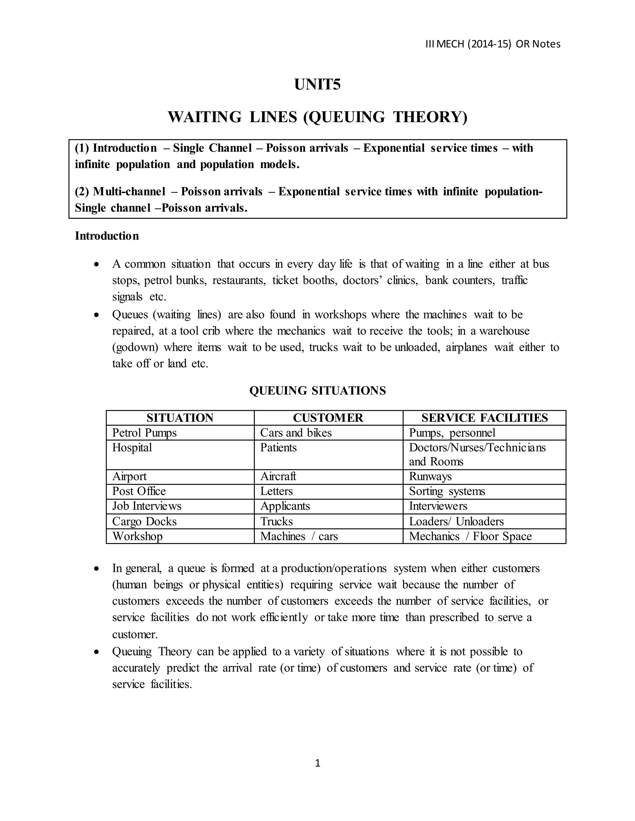
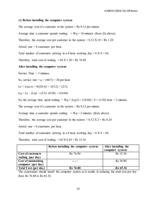
(3) Value of time both for customers and servers
(a) P0 = Probability of no customer in the system (or Probability system is idle) = [1-(λ/µ)]
(b) Pw = Probability that an arriving customer has to wait before being served = 1-P0 = (λ/µ)
(c) Pn = Probability of n customers waiting for service in the queuing system = P0 . (λ/µ)n
= [1-(λ/µ)]. (λ/µ)n
(d) ρ = System Utilization = Percentage of time a server is busy serving the customers = (λ/µ)
(e) P (T > t) = Probability being in the system (Waiting and being served) for more than time t
= e- (µ-λ)λt
(f) P (T ≤ t) = (Probability being in the system (Waiting and being served) for less than or
equal to time t) = 1- P (T > t).
(g) P (n > r) = Probability that the number of customers in the system, n exceeds a given
number, r = ((λ/µ)r+1
(h) Expected length of non-empty queue = [µ/(µ - λ)]
PROBLEMS ON QUEUING
SINGLE SERVER QUEUING MODELS
Q (1) For a queuing system, the arrival rate of calling population is 8 per hour. The service rate
is 12 per hour. Find all performance measures for the system.
Solution
Given :
Average arrival rate per hour = λ = 8
Average service rate = µ = 12
(i) Ls = Average number of customers in the system = [λ/(µ - λ)] = [8/(12-8)]
= (8/4) = 2

9. IIIMECH (2014-15) OR Notes
9
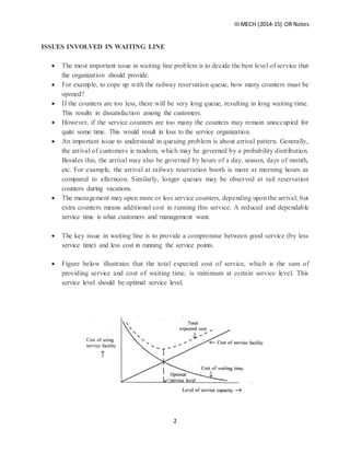
(ii) Lq = Average number of customers waiting for service in the queue = Ls – (λ/µ) =
[2-(8/12] = (4/3)
(iii) Wq = Average time an arriving customer has to wait in the queue before being served
= (Lq / λ) = (4/3) (1/8) = (1/6) hour = 10 minutes
(iv) Ws = Average time an arriving customer spends in the system = (Ls / λ) = (2/8)
= (1/4) hour = 15 minutes
(v) P0 = Probability of no customer in the system (or Probability system is idle)
= [1-(λ/µ)] = [1-(8/12)] = [1-(2/3)] = (1/3)
(vi) Pw = Probability that an arriving customer has to wait before being served
= 1-P0 = (λ/µ) = (8/12) = (2/3)
(vii) Pn = Probability of exactly 3 customers waiting for service in the queuing system
= P0 . (λ/µ)n = (1/3). (8/12)3 = 0.0988
(viii) ρ = System Utilization = Percentage of time a server is busy serving the customers
= (λ/µ) = (8/12) = (2/3)
(ix)P (T > t) = Probability being in the system (Waiting and being served) for more than 5
minutes (= 1/12 hours) = e- (µ-λ)λt = e- (12-8) 8 .(1/12)= 0.0694
Q (2) A TV repairman finds that the time spent on his jobs has an exponential distribution with
mean 30 minutes. If he repairs sets in the order in which they come in and if the arrival of sets
approximately is Poisson with an average rate of 10 per an 8 hour day, what is the repairman’s
expected idle time each day? How many jobs are ahead of the average TV just brought in?
Solution
Arrival rate = λ = 10 per day of 8 hours = (10/8) = 1.25 per hour.
Service time = (1/µ) = 30 minutes = (1/2) hour
Therefore, Service rate = µ = 2 per hour.
(a) Expected idle time of repairman
Probability system is busy = (λ/µ) = (1.25/2) = 0.625
Therefore, repairman is busy in a 8 hours day = 8 X 0.625 = 5 hours.
Therefore, the repairman is idle for 8-5 = 3 hours.
(b) Number of sets ahead of the TV set just brought in
Average number of customers in the system = [λ/(µ - λ)] = [1.25/(2-1.25)] = 1.667
Thus, there are 1.667 TV sets in the system ahead of the TV set just brought in.

10. IIIMECH (2014-15) OR Notes
10
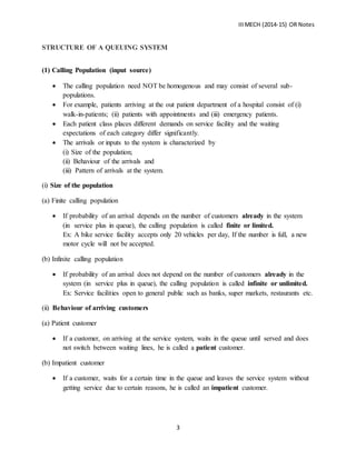
Q (3) In a railway marshalling yard, goods trains arrive at a rate of 30 trains per day. Assuming
that the inter-arrival time follows a Poisson distribution and the service time (the time taken to
hump a train) distribution is exponential with an average of 36 minutes.
Calculate:
(a) Expected queue size (line length)
(b) Probability that the queue size exceeds 10.
If the input of trains increases to an average of 33 per day, what will be the change in (a) and (b)?
Solution
(a) Expected queue length
Arrival rate λ = 30 trains per day = (30/24) = 1.25 per hour.
Service time = 36 minutes = (36/60) hours
Service rate = (1/Service time) = (60/36) = (5/3) = 1.667 per hour
Average number of trains in the system = [λ/(µ - λ)] = [1.25/(1.667-1.25)] = (1.25/0.417) = 3
So, expected queue length = Average number of trains waiting to be served = Ls – (λ/µ)
= 3-(1.25/1.667) = 2.25 trains.
(b) Probability that the queue size exceeds10
Probability that the queue size exceeds 10 = P (n > r) = ((λ/µ)r+1= (1.25/1.667)(10+1) = 0.0422
IF THE ARRIVAL RATE INCREASES TO 33 PER DAY,
(a) Expected queue length
Arrival rate λ = 33 trains per day = (33/24) = 1.375 per hour.
Service time = 36 minutes = (36/60) hours
Service rate = (1/Service time) = (60/36) = (5/3) = 1.667 per hour
Average number of trains in the system = [λ/(µ - λ)] = [1.375/(1.667-1.375)]
= (1.25/0.292) = 4.71
So, expected queue length = Average number of trains waiting to be served = Ls – (λ/µ)
= 4.71- (1.375/1.667) = 3.885 trains.
(b) Probability that the queue size exceeds10
Probability that the queue size exceeds 10 = P (n > r) = ((λ/µ)r+1= (1.375/1.667)(10+1) = 0.1202

11. IIIMECH (2014-15) OR Notes
11
Q (4) Telephone users arrive at a booth following a Poisson distribution with an average time of
10 minutes between one arrival and the next. The time taken for a telephone call is on an average
3 minutes and it follows an exponential distribution.
(a) What is the probability that a person arriving at the booth will have to wait?
(b) The telephone booth will install a second booth when convinced that an arrival would expect
waiting for at least 3 minutes for a phone call. By how much should the flow of arrivals increase
in order to justify a second booth? (c) What is the average length of the queue that forms from
time to time? (d) What is the probability that it will take a customer more than 5 minutes
altogether to wait for the phone and complete the call?
Solution
Given:
Inter-arrival time = 10 minutes = (1/6) hour.
Therefore, arrival rate per hour = λ = 6
Service time = 3 minutes = (1/20) hour
Therefore service rate per hour = µ = 20
(a) Probability that a person arriving has to wait = P (System is busy) = (λ/µ) = (6/20) = 0.30
(b) The second booth will be installed only if the expected waiting time is greater than or equal
to 3 minutes. i.e., Wq ≥ 3 minutes = (1/20) hour.
Therefore Wq = [λ’
/(µ (µ-λ’
))] ≥ (1/20)
So, [λ’
/(20 (20-λ’
))] ≥ (1/20).
λ’
≥ 10
Therefore, the arrival rate has to be greater than or equal to 10 customers per hour to justify a
second booth.
Hence the increase in the arrival rate has to be 4 customers (= 10-6) per hour.
(c) Average length of the queue that forms from time to time = Expected length of a non-empty
queue = [µ/(µ-λ)] = [20/(20-6)] = 1.429
(d) Probability that it will take a customer more than 5 minutes altogether to wait for the
phone and complete the call
Waiting time in the system = Waiting time in the queue to be served + Service Time.
In this problem, service time = 3 minutes.

12. IIIMECH (2014-15) OR Notes
12
Therefore Probability of waiting in the system for more than 5 minutes = Probability of waiting
in the queue for more than 2 minutes (=2/60 hour) = P (T > t) = e-( µ-λ)λt
= e-(20-6)6.(2/60)
=0.0608.
Q (5) A road transport company has one reservation clerk on duty at a time. He handles
information of bus schedules and makes reservations. Customers arrive at a rate of 8 per hour
and the clerk can, on an average serve 12 customers per hour.
After stating your assumptions, answer the following:
(a) What is the average number of customers waiting for the service of the clerk (number in the
system).
(b) What is the average time a customer has to wait before being served?
(c) What is the average time a customer spends in the system?
(d) The management is contemplating the installation of a computer system for handling
information and reservation. This is expected to reduce the service time from 5 minutes to 3
minutes. The additional cost of having the system works out to Rs 50 per day. If the cost of
goodwill of having to wait is estimated to be 12 paise per minute spent waiting before being
served, should the company install the computer system? Assume an 8-hour working day.
Solution
Given:
Average arrival rate = λ = 8 per hour.
Average service time = 5 minutes
So, average service rate = µ = (60/5) = 12 per hour
(a) Average number of customers waiting for the service of the clerk (number in the system) =
Ls = λ/(µ-λ) = 8/(12-8) = (8/4) = 2.
(b) Average time a customer spends in the queue before being served = Wq
Wq = (Lq/λ)
Lq = Ls – (λ/µ) = 2- (8/12) = (16/12) = (4/3)
Wq = (Lq/λ) = (4/3) / 8 = (1/6) hour = 10 minutes
(c) The average time a customer spends in the system= Ws = Ls/λ = 2/8 =(1/4) hour = 15
minutes.

13. IIIMECH (2014-15) OR Notes
13
(d) Before installing the computer system
The average cost of a customer in the system = Rs 0.12 per minute.
Average time a customer spends waiting = Wq = 10 minutes (from (b) above).
Therefore, the average cost per customer in the system = 0.12 X 10 = Rs 1.20
Arrival rate = 8 customers per hour.
Total number of customers arriving in a 8 hour working day = 8 X 8 = 64.
Therefore, total cost of waiting = 64 X 1.20 = Rs 76.80
After installing the computer system
Service Time = 3 minutes.
So, service rate = µ = (60/3) = 20 per hour.
Ls = λ/(µ-λ) = 8/(20-8) = (8/12) = (2/3).
Lq = Ls – (λ/µ) = (2/3)- (8/20) = (16/60)
So, the average time spent waiting = Wq = (Lq/λ) = (16/60) / 8 = (1/30) hour = 2 minutes
The average cost of a customer in the system = Rs 0.12 per minute.
Average time a customer spends waiting = Wq = 2 minutes (from above).
Therefore, the average cost per customer in the system = 0.12 X 2 = Rs 0.24
Arrival rate = 8 customers per hour.
Total number of customers arriving in a 8 hour working day = 8 X 8 = 64.
Therefore, total cost of waiting = 64 X 0.24 = Rs 15.36
Before installing the computer system After installing the
computer system
Cost of customers
waiting (per day)
Rs 76.80 Rs 15.36
Cost of maintaining
computer (per day)
----- Rs 50.00
Total Cost (per day) Rs 76.80 Rs 65.36
The corporation should install the computer system as it results in reducing the total cost per day
from Rs 76.80 to Rs 65.36.

14. IIIMECH (2014-15) OR Notes
14
Q (6) Customers arrive at the first class ticket counter of a theater at a rate of 12 per hour. There
is one clerk serving the customers at the rate of 30 per hour.
(a) What is the probability that there is no customer in the counter?
(b) What is the probability that there are more than 2 customers in the counter?
Solution
Given:
Arrival rate = λ = 12 per hour
Service rate = µ = 30 per hour.
(a) Probability (No customer in the system) = P0 = 1-(λ/µ) = 1-(12/30) = 0.60
(b) Probability (More than two customers in the system) = (λ/µ)n+1
= (12/30)(2+1) = (0.40)3 =
0.064.