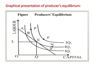
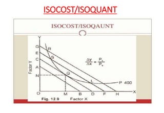
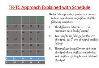
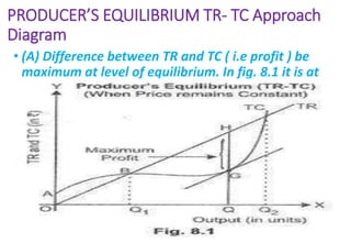
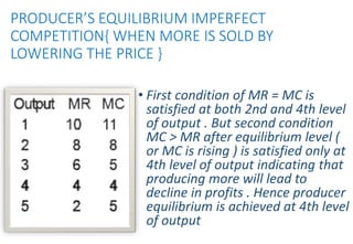
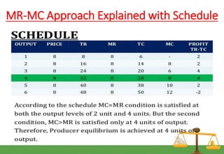
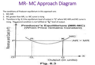
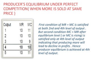
A producer seeks to maximize profits by producing at the level of output where marginal revenue equals marginal cost. This occurs at the producer's equilibrium. There are three main approaches to determining the producer's equilibrium: (1) where the isoquant is tangent to the isocost line, (2) where marginal revenue equals marginal cost, and (3) where the difference between total revenue and total cost is maximized. The equilibrium level of output is where profits are maximized and will fall if output increases beyond this level. Producer equilibrium can occur when price is constant, as in perfect competition, or when price decreases with increased output, as in imperfect competition.

1. PRODUCER
EQUILIBRIUM
MADE BY : NEERAJ GARWAL

3. Topic to be covered
1. Producer
2. Profit
3. Meaning and concept of producer’s equilibrium
4. Conditions of producer’s equilibrium
5. Producer equilibrium when price remain
Constant(PERFECT COMPETITION)
6. Producer equilibrium when price change/ fall
(IMPERFECT COMPETITION)

4. PRODUCEREQUILIBRIUM
Who is a “PRODUCER”?
A producer is an economic agent who
produces goods and services for sale
with the objective of
maximizing profit or minimizing
losses

5. PRODUCER’S EQUILIBRIUM
•It refers to a situation where producer
maximizes his profit or minimizes his
losses . It tells the level of output that
producer should undertake to produce to
achieve the objective of maximizing
profit and at this level of output there is
no incentive for firm either to increase or
decrease output

6. DISEQUILIBRIUM
• Disequilibriumcharacterizes a market that is not in equilibrium.Disequilibrium
can occur extremely briefly or over an extended period of time. Typically
in financial markets it either never occurs or only momentarily occurs, because
trading takes place continuously and the prices of financial assets can adjust
instantaneously with each trade to equilibrate supply and demand. At the other
extreme, many economists view labor markets as being in a state of
disequilibrium—specifically one of excess supply—over extended periods of
time. Goods markets are somewhere in between: prices of some goods, while
sluggish in adjusting due to menu costs, long term contracts, and other
impediments, do not stay at disequilibrium levels indefinitely, and many goods
markets such as commodity markets are highly organised and liquid and have
essentially instantaneous adjustment of their prices to equilibrium levels.

7. Isoquant-isocost Approach Of Producer
Equilibrium
1. To explain producer equilibrium, both
isoquants and isocost have to be analysed.
2. Producer equilibrium can be explain
graphically with the use of both isoquant
curve and isocost lines.
3. It is attained at the point where the isocost
line is tangent to the isoquant curve In the
graphs.

9. Isoquant
1. Isoquant is also called as equal product
curve or production indifference curve or
constant product curve.
2. Isoquant indicates various combinations of
two factors of production which give the
same level of output per unit of time.
3. The significance of factors of productive
resources is that, any two factors are
substitutable e.g. labour is substitutable for
capital and vice versa.

10. PROPERTIES OF ISOQUANT
The following are the main properties of isoquants:
1. Isoquants are downward sloping from left to right - Isoquant have a negative slope because if a firm wants
to employ more units of one factor, than it has to reduce the units of other factor to produce same level of
output. It is assumed that marginal product of the factors is positive i.e. increase in the quantity of factor
leads to positive increase in the output. Thus if the amount of one factor is increases, the amount of other
factor has to be decrease to produce the same level of output. There are certain inconsistencies follow if the
isoquants do not have a negative slope.
2. If the isoquant are upward sloping this means that the same quantity of output can be produced by
employing less units of both capital &labour i.e. marginal product of at least one factor is negative.
3.If the isoquant is parallel to Y axis this means that same quantity of output can be produced with the
same quantity of labour and any quantity of capital i.e. marginal product of capital is negative.
4.If the isoquant is parallel to X axis this means that same quantity of output can be produced with the
same quantity of capital and any quantity of labour i.e. marginal product of labour is negative.

11. Iso-costs
1. Isocost curve is the locus traced out by various
combinations of L and K, each of which costs
the producer the same amount of money (C )
Differentiating equation with respect to L, we
have dK/d. = -w/r
2. This gives the slope of the producer’s budget
line (isocost curve).
3. Isocost line shows various combinations of
labour and capital that the firm can buy for a
given factor prices.
4. The slope of iso cost line = PL/Pk. In this
equation , PL is the price of labour and Pk is the
price of capital. The slope of isocost line
indicates the ratio of the factor prices.

12. Profit maximization
1. Theisocost/isoquant method:
Profitis maximizedwhentheslopeof isoquantis equalto the
isocost.
2. Themarginalrevenue/marginalcostMethod:
At that output, MR(theslopeof Totalrevenuecurve) andMC(the
slopeof the totalcostcurve)areequal.
3. FromTR-TCapproach :
The difference between TR-TCis maximum

13. Graphical presentation of producer’s equilibrium:

14. ISOCOST/ISOQUANT

15. TR-TC Approach Explained with Schedule
OUT
PUT
AR TC TR PROF
IT
1 12 14 12 -2
2 12 26 24 -2
3 12 35 36 1`
4 12 52 48 -4
5 12 64 60 -4
Under this approach ,a producer is deemed
to be in equilibrium ,on fulfillment of the
following conditions
I. The difference between TR-TC is
maximum .(at 6 level of output)
II. Total profits are falling after this level
of output . (at 7 level of output profit is
falling)
III. The producer is equilibrium at 6 units
of output where profits are maximised
and profits are falling beyond this level
of output6 12 70 72 2
7 12 83 84 1

16. PRODUCER’S EQUILIBRIUM TR- TC Approach
Diagram
• (A) Difference between TR and TC ( i.e profit ) be
maximum at level of equilibrium. In fig. 8.1 it is at
“Q” level of output

17. PRODUCER’S EQUILIBRIUM IMPERFECT
COMPETITION{ WHEN MORE IS SOLD BY
LOWERING THE PRICE }
• First condition of MR = MC is
satisfied at both 2nd and 4th level
of output . But second condition
MC > MR after equilibrium level (
or MC is rising ) is satisfied only at
4th level of output indicating that
producing more will lead to
decline in profits . Hence producer
equilibrium is achieved at 4th level
of output

18. MR-MC Approach Explained with Schedule

19. MR- MC Approach Diagram
The conditions of Producer equilibrium in this approach are:
1. MC=MR
2. MC greater than MR, i.e. MC curve is rising
3. Therefore in fig. 8.3 the equilibrium level of output is “Q” where MC=MR and MC curve is
rising. The second condition is not fulfilled at “Q1” level of output.

20. PRODUCER’S EQUILIBRIUM UNDER PERFECT
COMPETITION{ WHEN MORE IS SOLD AT SAME
PRICE }
First condition of MR = MC is satisfied
at both 2nd and 4th level of output .
But second condition MC > MR after
equilibrium level ( or MC is rising) is
satisfied only at 4th level of output
indicating that producing more will
lead to decline in profits . Hence
producer equilibrium is achieved at 4th
level of output.

22. BIBLIOGRAPHY
1. Microeconomics: T.R.Jain & V.K.Ohri
2. Microeconomics: Sandeep Garg
3. All in One : Akansha Sharma
4. www.google.co.in=images+of+government+budget&chips=q:images+
of+government+MR
5. www.wikipedia.com
6. www.slideshare.com

23. THANK
YOU