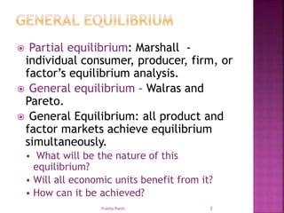
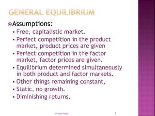
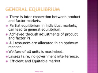
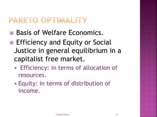
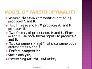
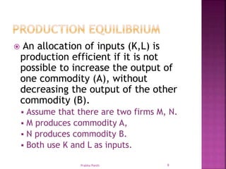
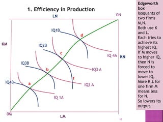
The document discusses general equilibrium theory and its key assumptions and implications. It addresses the following points in 3 sentences: General equilibrium theory posits that all markets, including both product and factor markets, will reach equilibrium simultaneously. This equilibrium will be Pareto optimal, meaning no individual can be made better off without making another worse off due to optimal resource allocation. The model assumes perfect competition, constant returns to scale, and that equilibrium is determined by price adjustments across interconnected markets.

1. Prof. Prabha Panth,
Osmania University,
Hyderabad

2.  Partial equilibrium: Marshall -
individual consumer, producer, firm, or
factor’s equilibrium analysis.
 General equilibrium – Walras and
Pareto.
 General Equilibrium: all product and
factor markets achieve equilibrium
simultaneously.
 What will be the nature of this
equilibrium?
 Will all economic units benefit from it?
 How can it be achieved?
Prabha Panth 2

3. Assumptions:
 Free, capitalistic market.
 Perfect competition in the product
market, product prices are given
 Perfect competition in the factor
market, factor prices are given.
 Equilibrium determined simultaneously
in both product and factor markets.
 Other things remaining constant,
 Static, no growth.
 Diminishing returns.
3Prabha Panth

4.  There is inter connection between product
and factor markets.
 Partial equilibrium in individual markets,
can lead to general equilibrium.
 Achieved through adjustments of product
and factor Ps.
 All resources are allocated in an optimum
manner.
 Welfare of all units is maximised.
 Laissez faire, no government interference.
 Efficient and Equitable market.
Prabha Panth 4

5.  Pareto Optimality: A Market situation,
where in it is not possible to make one
person better off, without making
another worse off.
 Because of Optimum allocation of
resources in General equilibrium.
 If resources are not allocated
optimally, it is possible to increase or
improve one unit’s welfare without
decreasing another’s.
Prabha Panth 5

6.  Basis of Welfare Economics.
 Efficiency and Equity or Social
Justice in general equilibrium in a
capitalist free market.
 Efficiency: in terms of allocation of
resources.
 Equity: in terms of distribution of
income.
Prabha Panth 6

7. Three conditions for Efficiency in the
General equilibrium model:
1. Production efficiency: Maximum
possible output with the given
resources.
2. Consumption efficiency: Maximum
utility for all consumers,
3. Product mix efficiency: optimum
mix of commodities.
Prabha Panth 7

8.  Assume that two commodities are being
produced A and B.
 Two firms M and N. M produces A, and N
produces B.
 Two factors of production, K and L. Firms
M and N use both factor inputs to produce A
and B.
 Two consumers X and Y, who consume both
commodities A and B.
 Perfect competition,
 Static analysis,
 Diminishing returns, and utility
Prabha Panth 8

9.  An allocation of inputs (K,L) is
production efficient if it is not
possible to increase the output of
one commodity (A), without
decreasing the output of the other
commodity (B).
 Assume that there are two firms M, N.
 M produces commodity A,
 N produces commodity B.
 Both use K and L as inputs.
Prabha Panth 9

10. 10
Edgeworth
box
Isoquants of
two firms
M,N.
Both use K
and L.
Each tries to
achieve its
highest IQ.
If M moves
to higher IQ,
then N is
forced to
move to
lower IQ.
More K,L for
one firm M
means less
for N.
So lowers its
output.
1. Efficiency in Production
0M
0N
IQ 1A
IQ2 A
IQ3 A
IQ 4A
LN
IQ2B
IQ3B
IQ4B
KM
IQ1B
LM
KN
a
b
c
d
f

11.  Edgeworth box: Diagrams of isoquants of
each individual firm M and N. Rotate that of
N, and align the two to form a box.
 Firm M’s isoquants are IQ1A, IQ2A, etc.
(purple lines)
 Firm N’s isoquants are IQ1B, IQ2B, etc. (blue
lines).
 OM is the origin for M, and ON is the origin
for N.
 Both firms compete for use of K and L.
 Each firm tries to reach its highest IQ.
 If M wants output of IQ4A, then N can
produce only IQ1B.
 If N wants to produce IQ4B, then M has to
produce IQ1A.
Prabha Panth 11

12.  At ‘f’ combination, M producing IQ2A,
while N is producing output of IQ2B.
 Is it possible to improve the situation?
 If they move to point ‘c’, then M can increase
output to IQ3A, and N can maintain its output
at IQ2B. (all combinations on the same IQ show
the same level of output).
 Now M is better off, but N is not worse off.
 Similarly, if they move to point ‘b’, then N’s
output increases to IQ3B, but M’s output
remains same at IQ2A as on point ‘f’.
 N is better off, but M is not worse off.
 Such adjustments called “Pareto
improvements” – when it is possible to improve
the welfare of one, without reducing another’s
welfare.
Prabha Panth 12

13.  At point b and c, IQ of both firms are
tangents to each other, (touch).
Similarly points a, b, c, and d.
Joining together these points, gives the
“Contact Curve” of production.
Moving along the contact curve leads to
improvement of one firm’s welfare
(output), but decreases the other’s
welfare (output).
Thus all points on the Contact curve are
“Pareto Optimal” points.
Prabha Panth 13

14.  At each of these points, a, b, c, d, the
slopes of their isoquants are the same.
 Also slopes of their isocost curves are
the same.
 We know that at equilibrium, slope of
isoquant = slope of isocost.
 Slopes of isoquants of M and N
= MRTSA = MRTSB
 Slope of isocost of K and L for the two firms:
= w/i
 At each of the equilibrium points ‘a b c d’ on
the contact curve,
= MRTSA = MRTSB = w/i
Prabha Panth 14

15.  Edgeworth box shows output of A and
B with isoquants in input factor space.
 To convert to output factor space, the
two goods should be shown on the two
axis (instead of K and L).
 Can be done using the Production
Possibility Curve (PPC), or the Product
Transformation Curve (PTC).
 The PPC shows the equilibrium outputs
of A and B with different inputs of K,L.
It is the transformation of the contract
curve on to the outer space.
Prabha Panth 15

16. 16
Transformation Curve
shows alternative
combinations of 2 goods
that can be produced
with given amounts of
factor inputs.
Points on Contact Curve
abcd of Figure 1, shown
in outer space.
As Q of A rises, Q of B
falls.
Inverse relationship.
PPC is convex outwards,
the slope increases with
increase in B.
Diminishing returns.
CommodityB
Commodity A
0
a
b
c
d
A
1
A
2
A
3
A
4
B1
B2
B3
B4
2. THE PRODUCTION
POSSIBILITY CURVE OR
TRANSFORMATION
CURVE

17.  The PPC shows how one good A is
transformed into another B, by
transferring resources from the
production of A to that of B.
1) PPC is concave to the origin: To produce
one more unit of B, more and more of A
should be given up. Shows diminishing
returns.
2) Slope of PPC: measures the Marginal
Rate of Product Transformation : MRPT
between the two goods.
Prabha Panth 17

18. MRPT of A, B, shows the amount by which
B has to fall, for A to rise, with the help
of resources released by reducing B.
MRPTA,B = - dA = MCB ----------- (1)
dB MCA
MRPT is the rate at which the economy
can transform one commodity into
another, through reallocation of K and L.
There is no unique Pareto optimum
situation.
All points on the PPC are Pareto optimum.
All points below the PPC are not efficient.
Prabha Panth 18

19. In P.C. firms equate P =
MC, so MCA = PA, MCB=
PB.
Slope of PPC = MRPTA,B
= dB = MCA = PA -----(2)
dA MCB PB
Given product prices,
production equilibrium is
the point where slope of
PPC = ratio of product Ps.
At point T on the
diagram.
CC is the Isocost curve,
whose slope = Pa/Pb
At T, OAT of A is produced
and OBt of B is produced.
Producers’ equilibrium,
and Product Efficiency
19
CommodityB
Commodity A
0
T
A2
B2
3. PRODUCT EFFICIENCYC
C

20. Prabha Panth 20