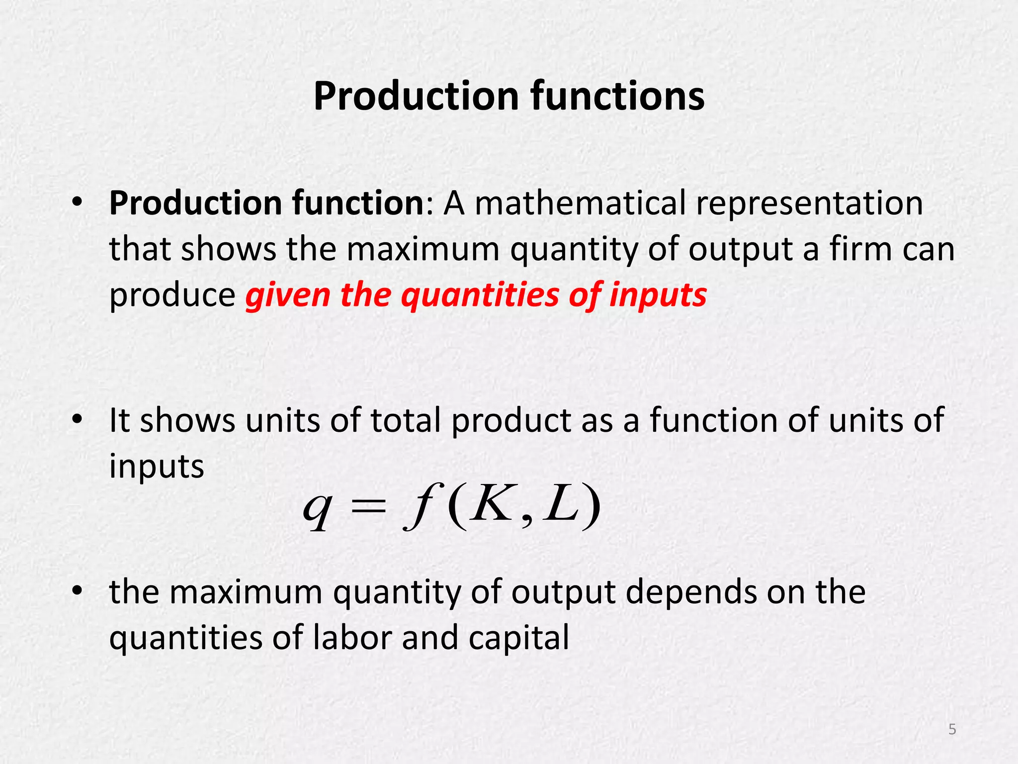
Production
Learning Objectives
After completing this session, students will be able to:
• Define Production Functions
• Differentiate Total, Marginal and Average Products
• Explain the Law of Diminishing Marginal Returns
• Describe an Isoquant and its properties
• Describe Production possibilities frontier
2
Production
• Production is the process by which inputs are
combined, transformed, and turned into
outputs
• An entrepreneur must put together resources -
- land, labour, capital -- and produce a product
• The productive resources, such as labor and
capital equipment, are called inputs or factors
of production
3
Production…
• Production technology refers to the quantitative
relationship between inputs and outputs
– A labor-intensive technology relies heavily on
human labor instead of capital
– A capital-intensive technology relies heavily on
capital instead of human labor
–Which input is more employed?
4
Production functions
• Production function: A mathematical representation
that shows the maximum quantity of output a firm can
produce given the quantities of inputs
• It shows units of total product as a function of units of
inputs
• the maximum quantity of output depends on the
quantities of labor and capital
5
)
,
( L
K
f
q 
Total, marginal and average product
• Total product (TP) is the whole amount of output
produced by all the factors employed
• Average product is the average amount produced
by each unit of a variable factor of production
• Average product is simply “output per worker”
6
averageproduct of labor =
total product
total units of labor L
Q
L
TP
AP 

Marginal product
• Marginal product (MP) is the additional output that can be
produced by adding one more unit of a specific input,
ceteris paribus
– MP of labor is the extra output obtained by employing
one more unit of labor while holding the level of capital
constant
7
marginal product of labor =
change in total product
change in units of labor used
1
1 


 





L
L L
Q
L
TP
MP
The law of diminishing marginal returns
• It is expected that the marginal product of an input
will depend upon the level of the input used
• Initially, output increases rapidly as new workers are
added, but eventually it diminishes as the fixed
capital becomes over utilized
• The law of diminishing marginal returns states that:
– When additional units of a variable input are
added to fixed inputs continuously, the marginal
product of the variable input finally declines,
ceteris paribus
8
The law of DMR…
• With a given amount of fixed factors, when one
worker is employed, he can use only some of the
fixed factors each time
• When more workers are employed, they can
specialize and raise the productivity – (MP & AP)
• However, after all the fixed factors have been
efficiently used, additional workers can help the
preceding workers only
– MP  which will finally drag down AP (even TP)
9
10
Production function…
• increasing marginal returns to labor: an increase in
the quantity of labor increases total output at an
increasing rate
– because of the gains from specialization of labor
(concentrate on the tasks)
• diminishing marginal returns to labor: an increase
in the quantity of labor still increases total output
but at a decreasing rate
11
Production function…
• diminishing total returns to labor: an increase in the
quantity of labor decreases total output
– diminishing total returns occur because of the
fixed size of factors: if the quantity of labor used
becomes too large, workers don’t have enough
space to work effectively
– also, as the number of workers employed in the
plant grows, their efforts become increasingly
difficult to coordinate
12
Total, average, and marginal product
• Marginal product is the slope of the
total product function
• At point A, the slope of the total
product function is highest; thus,
marginal product is highest
• At point C, total product is maximum,
the slope of the total product function
is zero, and marginal product intersects
the horizontal axis
• The marginal product of labor at any
point equals the slope of the total
product curve at that point
13
Production functions with a single input
Total, average, and marginal product
• The average product at any point
is equal to the slope of the ray
from the origin to the total
product curve at that point
• When a ray drawn from the origin
falls tangent to the total product
function, average product is
maximum and equal to marginal
product at that point
14
Total, average, and marginal product
• As long as marginal product rises,
average product rises
• When marginal product is greater
than average product, average
product rises
• When marginal product equals
average product, average product is
at its maximum
• When marginal product is less than
average product average product falls
15
Three stages of production
Stage Total product Marginal product
Average
product
I
Increases at an
increasing rate
Increases, reaches its
maximum & then
declines till MR = AP
Increases &
reaches its
maximum
II
Increases at a
diminishing rate
till it reaches max
Is diminishing and
becomes equal to zero
Starts
diminishing
III
Starts declining Becomes negative
Continues to
decline
16
Stages of production…
• From the above table only stage II is rational which
means relevant range for a rational firm to operate
• In stage I it is profitable for the firm to keep on
increasing the use of labour
• In stage III, MP is negative and hence it is inadvisable
to use additional labour
– I.e. Stage I and III are irrational
17
Isoquant
• An isoquant is a curve that shows the various
combinations of inputs that will produce the same (a
particular) amount of output
18
• The curve represents the technically
efficient combinations of staff time
and bicycles that can produce 1,000
units of output per period
Isoquant…
• An isoquant map is a contour map of a firm’s
production function
• All of the isoquants from a production function are part
of this isoquant map
• The isoquants labeled q =
2000 and q = 3000 represent
two more of the infinite curves
that represent different levels
of output
• the farther away from the
origin, levels of output
becomes higher
Isoquant…
• The slope of an isoquant has a technical name
called the marginal rate of technical
substitution (MRTS) or the marginal rate of
substitution in production
• Thus in terms of capital services K and labour L;
MRTS = K/ L
20
Properties of isoquants
a. An isoquant is downward sloping to the right
I.e. negatively inclined
– This implies that for the same level of output, the
quantity of one variable will have to be reduced in
order to increase the quantity of other variable
b. A higher isoquant represents larger output
– That is with the same quantity of one input and
larger quantity of the other input, larger output
will be produced
21
Properties...
c. No two isoquants intersect or touch each other
– If the two isoquants do touch or intersect that means
that a same amount of two inputs can produce two
different levels of output which is absurd
d. Isoquant is convex to the origin
– This means that the slope declines from left to right
along the curve
– That is when we go on increasing the quantity of one
input say labour by reducing the quantity of other
input say capital; we see less units of capital are
sacrificed for the additional units of labour
22
Economic and uneconomic regions
23
Economic and uneconomic regions…
• the isoquants now have upward-sloping and
backward-bending regions
• this correspond to a situation in which one input has
a negative marginal product, or what we called
diminishing total returns
• the upward-sloping region occurs because there are
diminishing total returns to labor (MPL < 0)
• the backward-bending region arises because of
diminishing total returns to capital (MPK < 0)
24
Economic and uneconomic regions…
• If we have diminishing total returns to labor, then as
we increase the quantity of labor, holding the
quantity of capital fixed, total output goes down
• Thus, to keep output constant (moving along an
isoquant), we must also increase the amount of
capital to compensate for the diminished total
returns to labor
• A firm that wants to minimize its production costs
should never operate in a region of upward-sloping
or backward-bending isoquants
26
Economic and uneconomic regions…
• Compare point A and E
• The firm could produce the same output but at a
lower cost by producing at point E
• By producing in the range where the marginal
product of labor is negative, the firm would be
wasting money by spending it on unproductive labor
• the economic region of production is the region of
downward-sloping isoquants
• the uneconomic region of production is the range in
which isoquants slope upward or bend backward
27
Production possibilities frontier (PPF)
• A graph that illustrates the
different combinations of
outputs that are achievable
with a limited set of resources
• Any point inside the curve –
suggests resources are not
being utilized efficiently and
any point outside the curve –
not attainable with the current
level of resources
28
PPF…
• Useful to demonstrate economic growth and
opportunity cost
• Assume a clinic can produce two types of outputs
with its resources – health care and other
commodities (food, education, transport)
• If it devotes all resources to health care it could
produce a maximum of 1500 units of health care
• If it devotes all its resources to other commodities it
could produce a maximum of 3600 units of other
commodities
29
Activity
1. Which of the points in the Figure (A, B, C and D) are:
A. Efficient?
B. Inefficient?
C. Not feasible?
30
2. What is the opportunity cost of increasing health
care from 500 to 1000 units?
a) starting from point A?
b) Starting from point B?
3. what you think would happen to the PPF if:
a) there is a decrease in the size of the labor force
b) there is an improvement in health technology
31

6. production

  • 1.
  • 2.
    Learning Objectives After completingthis session, students will be able to: • Define Production Functions • Differentiate Total, Marginal and Average Products • Explain the Law of Diminishing Marginal Returns • Describe an Isoquant and its properties • Describe Production possibilities frontier 2
  • 3.
    Production • Production isthe process by which inputs are combined, transformed, and turned into outputs • An entrepreneur must put together resources - - land, labour, capital -- and produce a product • The productive resources, such as labor and capital equipment, are called inputs or factors of production 3
  • 4.
    Production… • Production technologyrefers to the quantitative relationship between inputs and outputs – A labor-intensive technology relies heavily on human labor instead of capital – A capital-intensive technology relies heavily on capital instead of human labor –Which input is more employed? 4
  • 5.
    Production functions • Productionfunction: A mathematical representation that shows the maximum quantity of output a firm can produce given the quantities of inputs • It shows units of total product as a function of units of inputs • the maximum quantity of output depends on the quantities of labor and capital 5 ) , ( L K f q 
  • 6.
    Total, marginal andaverage product • Total product (TP) is the whole amount of output produced by all the factors employed • Average product is the average amount produced by each unit of a variable factor of production • Average product is simply “output per worker” 6 averageproduct of labor = total product total units of labor L Q L TP AP  
  • 7.
    Marginal product • Marginalproduct (MP) is the additional output that can be produced by adding one more unit of a specific input, ceteris paribus – MP of labor is the extra output obtained by employing one more unit of labor while holding the level of capital constant 7 marginal product of labor = change in total product change in units of labor used 1 1           L L L Q L TP MP
  • 8.
    The law ofdiminishing marginal returns • It is expected that the marginal product of an input will depend upon the level of the input used • Initially, output increases rapidly as new workers are added, but eventually it diminishes as the fixed capital becomes over utilized • The law of diminishing marginal returns states that: – When additional units of a variable input are added to fixed inputs continuously, the marginal product of the variable input finally declines, ceteris paribus 8
  • 9.
    The law ofDMR… • With a given amount of fixed factors, when one worker is employed, he can use only some of the fixed factors each time • When more workers are employed, they can specialize and raise the productivity – (MP & AP) • However, after all the fixed factors have been efficiently used, additional workers can help the preceding workers only – MP  which will finally drag down AP (even TP) 9
  • 10.
  • 11.
    Production function… • increasingmarginal returns to labor: an increase in the quantity of labor increases total output at an increasing rate – because of the gains from specialization of labor (concentrate on the tasks) • diminishing marginal returns to labor: an increase in the quantity of labor still increases total output but at a decreasing rate 11
  • 12.
    Production function… • diminishingtotal returns to labor: an increase in the quantity of labor decreases total output – diminishing total returns occur because of the fixed size of factors: if the quantity of labor used becomes too large, workers don’t have enough space to work effectively – also, as the number of workers employed in the plant grows, their efforts become increasingly difficult to coordinate 12
  • 13.
    Total, average, andmarginal product • Marginal product is the slope of the total product function • At point A, the slope of the total product function is highest; thus, marginal product is highest • At point C, total product is maximum, the slope of the total product function is zero, and marginal product intersects the horizontal axis • The marginal product of labor at any point equals the slope of the total product curve at that point 13 Production functions with a single input
  • 14.
    Total, average, andmarginal product • The average product at any point is equal to the slope of the ray from the origin to the total product curve at that point • When a ray drawn from the origin falls tangent to the total product function, average product is maximum and equal to marginal product at that point 14
  • 15.
    Total, average, andmarginal product • As long as marginal product rises, average product rises • When marginal product is greater than average product, average product rises • When marginal product equals average product, average product is at its maximum • When marginal product is less than average product average product falls 15
  • 16.
    Three stages ofproduction Stage Total product Marginal product Average product I Increases at an increasing rate Increases, reaches its maximum & then declines till MR = AP Increases & reaches its maximum II Increases at a diminishing rate till it reaches max Is diminishing and becomes equal to zero Starts diminishing III Starts declining Becomes negative Continues to decline 16
  • 17.
    Stages of production… •From the above table only stage II is rational which means relevant range for a rational firm to operate • In stage I it is profitable for the firm to keep on increasing the use of labour • In stage III, MP is negative and hence it is inadvisable to use additional labour – I.e. Stage I and III are irrational 17
  • 18.
    Isoquant • An isoquantis a curve that shows the various combinations of inputs that will produce the same (a particular) amount of output 18 • The curve represents the technically efficient combinations of staff time and bicycles that can produce 1,000 units of output per period
  • 19.
    Isoquant… • An isoquantmap is a contour map of a firm’s production function • All of the isoquants from a production function are part of this isoquant map • The isoquants labeled q = 2000 and q = 3000 represent two more of the infinite curves that represent different levels of output • the farther away from the origin, levels of output becomes higher
  • 20.
    Isoquant… • The slopeof an isoquant has a technical name called the marginal rate of technical substitution (MRTS) or the marginal rate of substitution in production • Thus in terms of capital services K and labour L; MRTS = K/ L 20
  • 21.
    Properties of isoquants a.An isoquant is downward sloping to the right I.e. negatively inclined – This implies that for the same level of output, the quantity of one variable will have to be reduced in order to increase the quantity of other variable b. A higher isoquant represents larger output – That is with the same quantity of one input and larger quantity of the other input, larger output will be produced 21
  • 22.
    Properties... c. No twoisoquants intersect or touch each other – If the two isoquants do touch or intersect that means that a same amount of two inputs can produce two different levels of output which is absurd d. Isoquant is convex to the origin – This means that the slope declines from left to right along the curve – That is when we go on increasing the quantity of one input say labour by reducing the quantity of other input say capital; we see less units of capital are sacrificed for the additional units of labour 22
  • 23.
  • 24.
    Economic and uneconomicregions… • the isoquants now have upward-sloping and backward-bending regions • this correspond to a situation in which one input has a negative marginal product, or what we called diminishing total returns • the upward-sloping region occurs because there are diminishing total returns to labor (MPL < 0) • the backward-bending region arises because of diminishing total returns to capital (MPK < 0) 24
  • 26.
    Economic and uneconomicregions… • If we have diminishing total returns to labor, then as we increase the quantity of labor, holding the quantity of capital fixed, total output goes down • Thus, to keep output constant (moving along an isoquant), we must also increase the amount of capital to compensate for the diminished total returns to labor • A firm that wants to minimize its production costs should never operate in a region of upward-sloping or backward-bending isoquants 26
  • 27.
    Economic and uneconomicregions… • Compare point A and E • The firm could produce the same output but at a lower cost by producing at point E • By producing in the range where the marginal product of labor is negative, the firm would be wasting money by spending it on unproductive labor • the economic region of production is the region of downward-sloping isoquants • the uneconomic region of production is the range in which isoquants slope upward or bend backward 27
  • 28.
    Production possibilities frontier(PPF) • A graph that illustrates the different combinations of outputs that are achievable with a limited set of resources • Any point inside the curve – suggests resources are not being utilized efficiently and any point outside the curve – not attainable with the current level of resources 28
  • 29.
    PPF… • Useful todemonstrate economic growth and opportunity cost • Assume a clinic can produce two types of outputs with its resources – health care and other commodities (food, education, transport) • If it devotes all resources to health care it could produce a maximum of 1500 units of health care • If it devotes all its resources to other commodities it could produce a maximum of 3600 units of other commodities 29
  • 30.
    Activity 1. Which ofthe points in the Figure (A, B, C and D) are: A. Efficient? B. Inefficient? C. Not feasible? 30
  • 31.
    2. What isthe opportunity cost of increasing health care from 500 to 1000 units? a) starting from point A? b) Starting from point B? 3. what you think would happen to the PPF if: a) there is a decrease in the size of the labor force b) there is an improvement in health technology 31