1. Society consumes trillions upon trillions of petroleum in barrels every month. The question at
hand is whether or not our consumption follows a pattern. In fact it does! Presented in the data is the
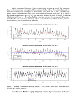
total amount of petroleum consumption by the residential sector, from 1984 to 2013. Figure 1 clearly
shows that our consumption fluctuates above and below the overall mean of our data! So by plotting a
Loess curve we are able to visibly see the rising and falling trends of our data! To remedy this trend we
take the first difference as well as a log, the latter as a means to reduce the varying scale of our data,
and behold the data is very much stationary, as there is very little fluctuation from the mean, which is
exactly what we need for our data to be stationary!
Now what model should we employ to represent our data? Figure two contains the ACF and
Figure 1: The RAW, Transformed, and Transformed + First Difference of our data. Notice how trend
becomes less and less apparent!
2. the PACF plots of our transformed and differenced data, and quite clearly we can see that neither an
auto regressive model nor would a moving average model be able to represent our model, so we must
use an ARMA model, and because we have taken a first difference we must employ the use of an
ARIMA(q,d,p) model! Using R's forecast package I employ the use of auto.arima() function to
determine our parameters, which come out to be ARIMA(5,1,4).
We now have a model to fit our data to! The next step to see if this model fits very well is to
perform a number of diagnostics to ensure our model is a good fit! First we look at the ACF and PACF
of our residuals, and there happen to significant values at particular lags, which tells me that the 5,1,4
model may not have been the best model to represent our data. Next we look to see if our residuals
fluctuate about a mean of 0, and quite certainly they in fact do. The next question is: are the residuals
normal and independent? The normal plot shows that they are indeed normal, and the Box-Ljung test
gives us a significantly large p-test (p = .94), which implies that our residuals are independent.
Figure 2: The ACF and PACF of our transformed and differenced data, notice that both do not cut off.
Implying that an ARMA model is appropriate! We also have our periodogram of our data! Notice that
a large peak occurs around .833! This is our frequency which relates to a cycle of 1.2 months!
3. However do take notice of the Ljung-Box test plot clearly shows that after two lags our model no
longer shows independent residuals. What does this mean? It implies any lag higher than two may be
of poor representation, in other words our model is only decent at examining two future values. Figure
three represent our conclusions graphically. Our results on the residuals are as follows:
1. Independent for lags up to 2
2. Constant variance
3. Fluctuate about mean
4. Residuals are normal
Our residuals do not represent only white noise, there are other errors being accounted for. So the
question is now then how effective is our model in predicting our future consumption of petroleum?
Using our suggested model, ARIMA(5,1,4) we attempt to predict the last 12 months of our
Figure 3: Our residual lots concerning residual analysis for our model. Notice how our model fails the
Ljung Box test and clearly shows significant values in it's ACF and PACF! This implies our model is
not the BEST!
4. observed data. Figure 4 shows our forecasted values, our observed values, as well as our prediction
bands (our standard error.) Our predicted values are actually quite spot on! Our observed and
forecasted values are well within range of one another and lie within our prediction bands, so our
model, ARIMA(5,1,4) turned out to be a decent fit for representing future values!
Using time series methods we observed that we were able to draw successful predictions to how
much petroleum the residential sector will consume per month! This example shows time series's
effectiveness in predicting the future. However what I must take note of is that our prediction were for
the next year only, not the year afterward or the year after that one. What should be taken with a grain
of salt is that though we can successfully predict the future to a relatively good degree, we are still
unable to account for possibly shocks in the future with the methods presented here. FIGURE clearly
shows how large our room for error is! Nevertheless time series remains to be a powerful tool in
predicting the future based on past observations.
Figure 4: Our predicted values and the observed values. Take note of how well our model actually
predicted the values!
5. Figure 6: Our periodogram of our final model, notice that it still retains the same significant frequency
(.899), which is made even more apparent in it's smoothed counter part!
6. Explicit R Code & Output:
> data <- read.table("Data.txt", header = TRUE)
>
> #Determine if the Series is stationary.
>
> #Plot the original data
> par(mfrow=(c(3,1)))
> Petro <- data$Petro
> Count = (1:359)
>
> plot(Petro~Count, type = "l",main = "Petriolium Consumed Be Residential Sector (Trillions) 1984 -
2013", ylab = "Original Petrolium")
> fitO = loess(Petro~Count, span = .25, family = "gaussian")
> lines(Count,fitO$fitted,col="red")
> abline(h = mean(Petro), col = 'blue')
> legend(0,100, c("Observed", "Loess", "Mean"), lty = c(1,1), lwd=c(2.5,2.5),col = c("black","red",
"blue"))
>
> #Transform the Data
> transData <- log(Petro)
> plot(transData ~ Count, type = "l", main = "Petriolium Consumed Be Residential Sector (Trillions)
1984 - 2013",ylab = "Log Petrolium")
> fitL = loess(transData ~ Count, span = .25, family = "gaussian")
> lines(Count,fitL$fitted,col="red")
> abline(h = mean(transData), col = 'blue')
> legend(0,4.4, c("Observed", "Loess", "Mean"), lty = c(1,1), lwd=c(2.5,2.5),col = c("black","red",
"blue"))
>
> #Take the First difference
> transDif <- diff(transData,differences=1)
> newCount = (1:358)
>
> #Plot the transformed data.
> plot(transDif~newCount, type = "l", main = "Petriolium Consumed Be Residential Sector (Trillions)
1984 - 2013",ylab = "First Difference Petrolium")
> fitD = loess(transDif ~ newCount, span = .25, family = "gaussian")
> lines(newCount,fitD$fitted,col="red")
> abline(h = mean(transDif), col = 'blue')
> legend(100,-.2, c("Observed", "Loess", "Mean"), lty = c(1,1), lwd=c(2.5,2.5),col = c("black","red",
"blue"))
>
> #This will make our Data stationary.
> #I will choose the Log + first difference of the Data.
> par(mfrow=c(2,2))
> acf (transDif, lag = 400)
> pacf (transDif, lag = 400)
> dataPeriod <-spec.pgram(transDif, taper = 0, fast=FALSE, detrend=FALSE,demean
8. > library('forecast')
Loading required package: zoo
Attaching package: ‘zoo’
The following objects are masked from ‘package:base’:
as.Date, as.Date.numeric
Loading required package: timeDate
This is forecast 5.2
> library('astsa')
> library("FitAR")
Loading required package: lattice
Loading required package: leaps
Loading required package: ltsa
Loading required package: bestglm
Loading required package: lars
Loaded lars 1.2
Loading required package: ElemStatLearn
Attaching package: ‘FitAR’
The following object is masked from ‘package:forecast’:
BoxCox
>
> #I choose an ARIMA model, d = 0 since the data is already differenced.
>
> #Select the final model using ID Criterion
> auto.arima(transDif, max.p = 8, max.q = 8, stationary = TRUE, ic = c("aicc", "aic", "bic"), trace =
TRUE)
ARIMA(2,0,2) with non-zero mean : -439.6081
ARIMA(0,0,0) with non-zero mean : -390.096
ARIMA(1,0,0) with non-zero mean : -414.5041
ARIMA(0,0,1) with non-zero mean : -401.6552
ARIMA(1,0,2) with non-zero mean : -435.8972
ARIMA(3,0,2) with non-zero mean : -590.5202
ARIMA(3,0,1) with non-zero mean : -553.3992
ARIMA(3,0,3) with non-zero mean : -624.6525
ARIMA(4,0,4) with non-zero mean : -641.8194
ARIMA(4,0,4) with zero mean : -643.3304
ARIMA(3,0,4) with zero mean : 1e+20
ARIMA(5,0,4) with zero mean : -654.9737
ARIMA(5,0,3) with zero mean : -636.1066
9. ARIMA(5,0,5) with zero mean : -629.8412
ARIMA(4,0,3) with zero mean : -636.4764
ARIMA(6,0,5) with zero mean : 1e+20
ARIMA(5,0,4) with non-zero mean : -653.4301
ARIMA(6,0,4) with zero mean : 1e+20
Best model: ARIMA(5,0,4) with zero mean
Series: transDif
ARIMA(5,0,4) with zero mean
Coefficients:
ar1 ar2 ar3 ar4 ar5 ma1 ma2 ma3 ma4
-0.2040 1.0071 0.1723 -0.9667 -0.1743 -0.0248 -1.2324 -0.1158 0.8848
s.e. 0.0613 0.0171 0.0601 0.0152 0.0599 0.0335 0.0319 0.0293 0.0282
sigma^2 estimated as 0.008753: log likelihood=336.29
AIC=-652.58 AICc=-651.95 BIC=-613.78
>
> #My model is going to be of order (5,1,4)
>
>
> #Perform residual analysis, show that our model is good. Make sure our error is white noise.
> par(mfrow = c(4,2))
>
> #Plot of Residuals
> fit <- Arima(transDif, order = c(5,0,4))
> plot(fit$residual, type = "p")
>
> abline(h=0, col = "red")
>
> #Normally Distributed?
> hist(fit$residuals)
>
> #AutoCorrelations present?
> acf(fit$residuals)
> pacf(fit$residuals)
>
> #Are they Normal?
> qqnorm(fit$residuals)
>
> #Does the Test say it is a good fit?
> Box.test(fit$residuals, type = c("Ljung-Box"))
Box-Ljung test
data: fit$residuals
X-squared = 0.0056, df = 1, p-value = 0.9402
10. > LBQPlot(fit$residuals, lag.max = 30)
> mean(fit$res)
[1] -0.001070552
>
> #Smoothed periodgram of residuals
> k = kernel("modified.daniell", c(6,6))
> spec.pgram(fit$residuals, k, taper=0, detrend=FALSE, demean=TRUE, log="no")
>
>
> par(mfrow = c(2,1))
> #Plot Spec Density of the Final MOdel as well as the Smoothed
> finalModel <- fitted(fit)
> spec.pgram(finalModel, taper = 0, fast=FALSE, detrend=FALSE,demean =TRUE,log="no")
> k = kernel("modified.daniell", c(6,6))
> spec.pgram(finalModel, k, taper=0, detrend=FALSE, demean=TRUE, log="no")
>
> #Refit The final model
>
> refit <- Arima(Petro[1:348], order = c(5,1,4))
> pred <- predict(refit, n.ahead = 12, d =1)
> pred$pred
Time Series:
Start = 349
End = 360
Frequency = 1
[1] 96.98064 96.96685 94.07727 82.66665 75.30919 63.93817 59.73830 59.37145 62.29238 72.78900
79.44755 90.20105
> pred$pred + pred$se
Time Series:
Start = 349
End = 360
Frequency = 1
[1] 109.44587 112.64558 111.26915 100.66319 93.42068 82.07828 77.88662 77.55500 80.87230
92.11042 100.52580 113.21682
> forePlus <- c(109.44587, 112.64558 ,111.26915 ,100.66319 , 93.42068 , 82.07828 , 77.88662,
77.55500, 80.87230 , 92.11042 ,100.52580, 113.21682)
>
> pred$pred - pred$se
Time Series:
Start = 349
End = 360
Frequency = 1
[1] 84.51540 81.28813 76.88539 64.67011 57.19769 45.79806 41.58997 41.18790 43.71247 53.46758
58.36930 67.18528
> foreMins <- c(84.51540, 81.28813, 76.88539, 64.67011, 57.19769, 45.79806, 41.58997 ,41.18790,
43.71247, 53.46758 ,58.36930 ,67.18528)
>
> index <- c(348:359)
> fore <- c(96.98064 ,96.96685, 94.07727, 82.66665, 75.30919, 63.93817, 59.73830, 59.37145,
11. 62.29238, 72.78900, 79.44755, 90.20105)
> par(mfrow=c(2,1))
> which.max(fore)
[1] 1
>
> par(mfrow = c(1,1))
>
> plot(Petro[348:359]~index, type = 'l', col = 'black', main = 'Plot of Forecasted and Observed Values',
xlab = "Time", ylab = "Petrolium Consumption", ylim = c(35,130))
> lines(fore~index, col = "red")
> lines(forePlus~index, col = "blue")
> lines(foreMins~index, col = "blue")
> legend(348,130, c("Observed","Predicted", "Prediction Bands"), lty = c(1,1), lwd=c(2.5,2.5),col =
c("black","red", "blue"))