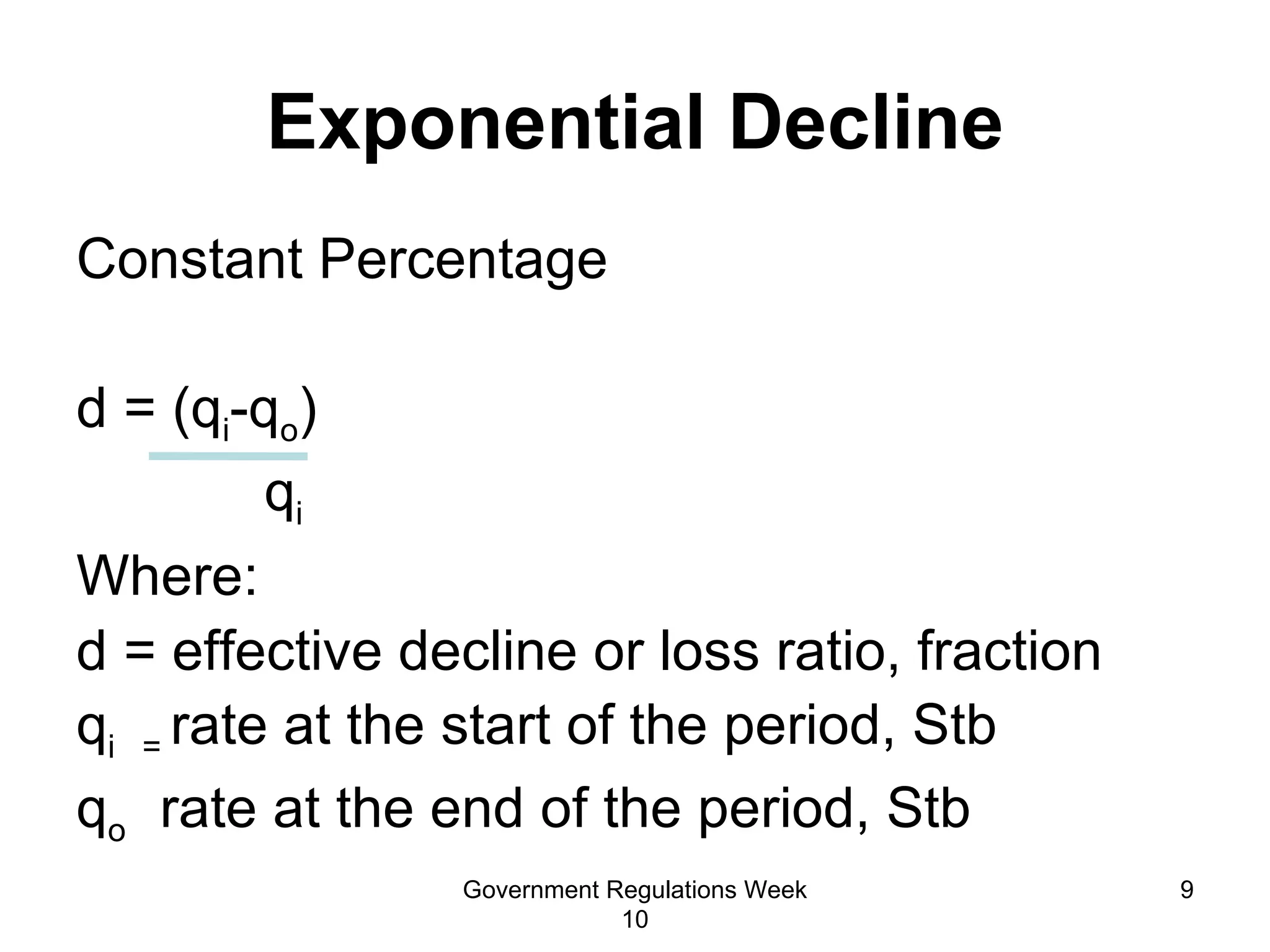
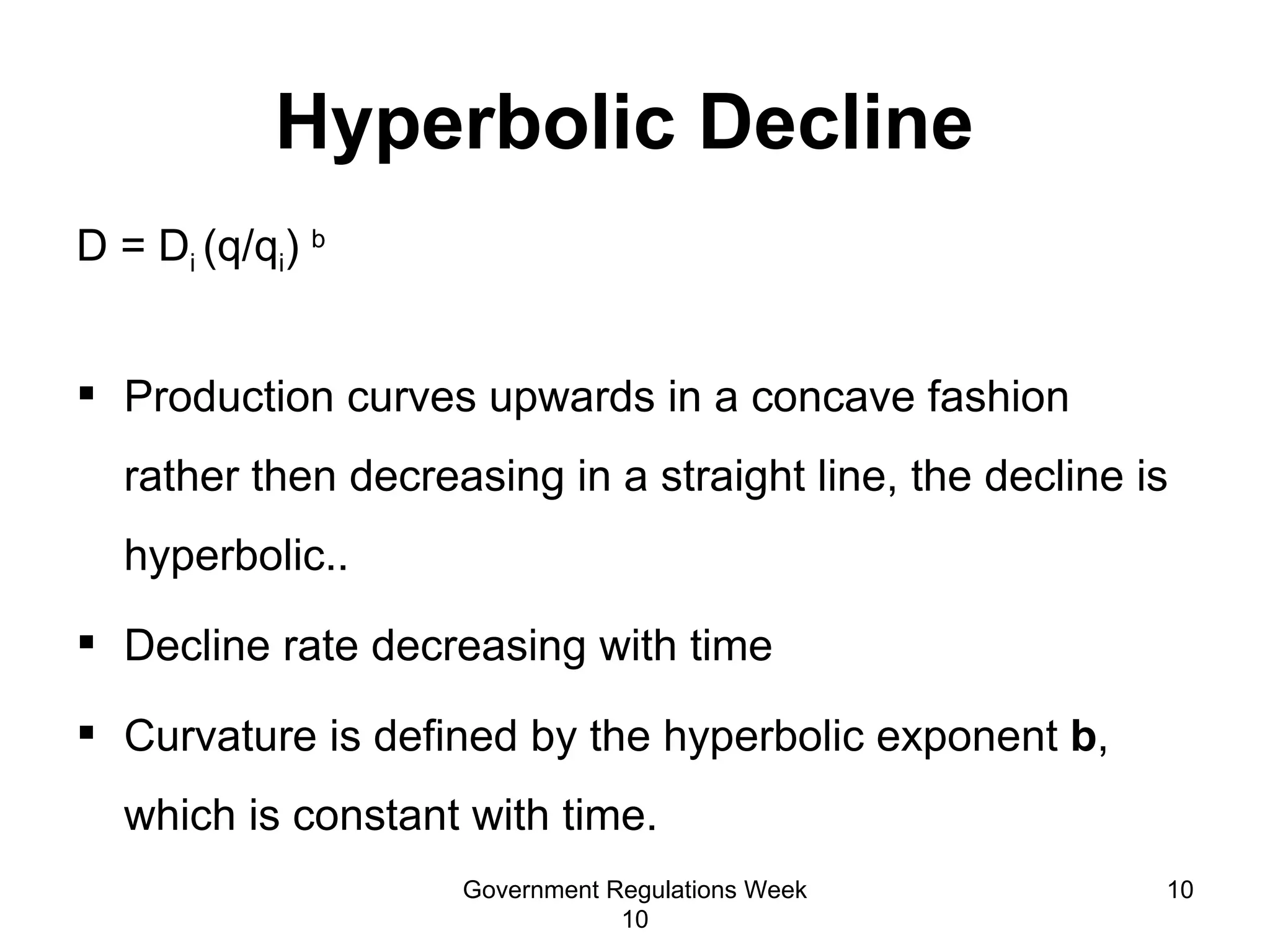
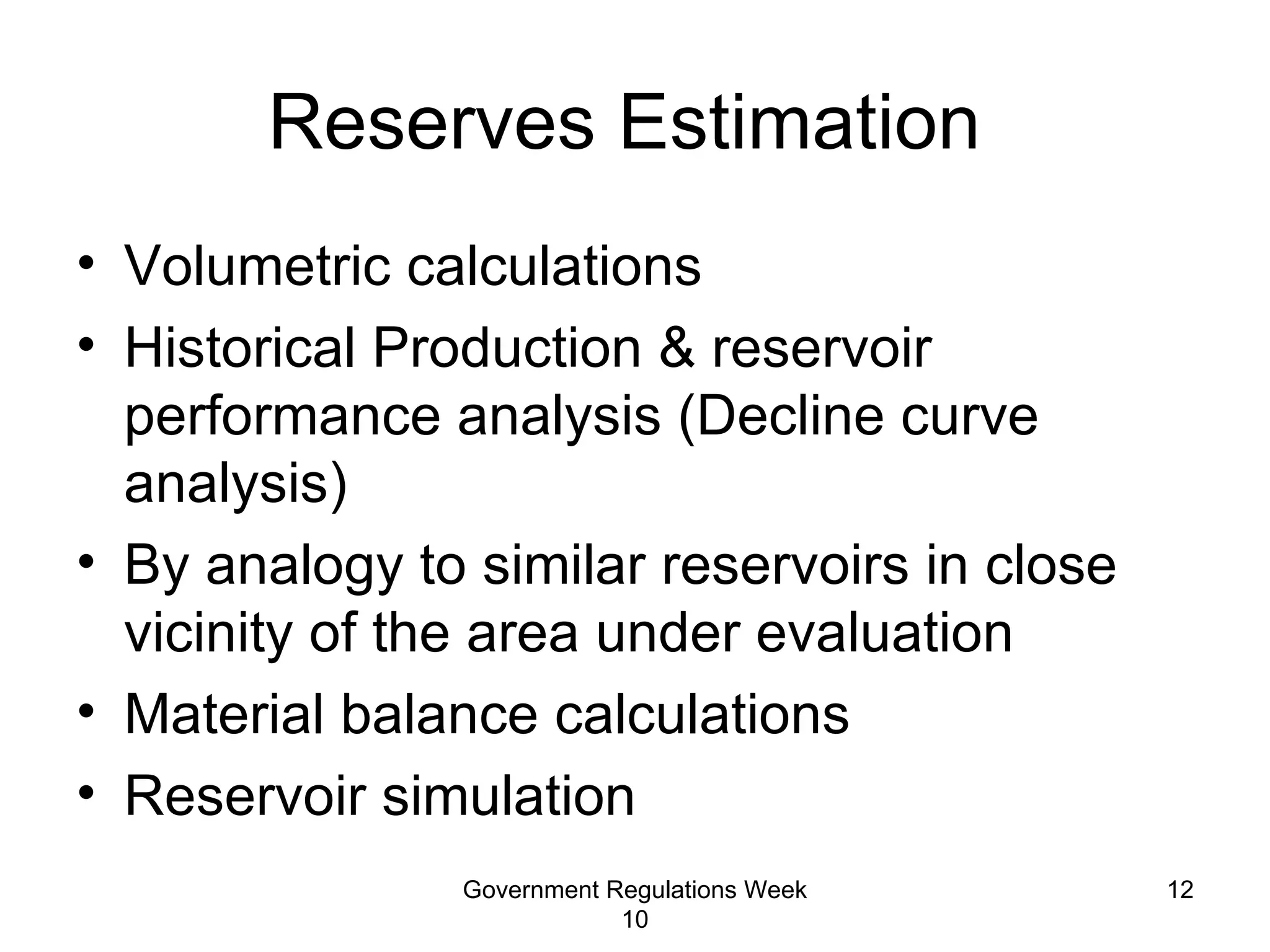
The document discusses definitions and categories of petroleum reserves based on probabilities of production. It defines proven, probable, and possible reserves, which have 90%, 50%, and 10% certainty of being produced, respectively. Methods for estimating reserves are described, including volumetric analysis, decline curve analysis, and production forecasting based on projected prices, costs, and other factors.

1. Petroleum Project Economics Econ210D Presentation 10 Government Regulations Week 10

2. Definition of reserves Reserves are an estimate of hydrocarbons existing and being producible under current economic conditions and technology. There are three categories of reserves based on different probabilities or degrees of certainty. Government Regulations Week 10

3. Proven reserves This is defined as oil and gas "Reasonably Certain" to be producible using current technology at current prices, with current commercial terms and government consent- Some Industry specialists refer to this as P90 - i.e having a 90% certainty of being produced. This is also known in the industry as 1P. Government Regulations Week 10

4. Probable reserves These are defined as oil and gas "Reasonably Probable" of being produced using current or likely technology at current prices, with current commercial terms and government consent. Some Industry specialists refer to this as P50 - i.e having a 50% certainty of being produced. This is also known in the industry as 2P or Proven plus probable. Government Regulations Week 10

5. Possible reserves This refers to reserves that have a chance of being developed under favourable circumstances" Some industry specialists refer to this as P10 - i.e having a 10% certainty of being produced. This is also known in the industry as 3P or Proven plus probable plus possible. Government Regulations Week 10

6. Proven reserves can be further categorized as follows: Proved Developed Producing Proved Developed Non-Producing Proved Undeveloped Proven Reserve Categories Government Regulations Week 10

7. Structure maps & cross sections Well logs Core Analysis Fluid Data Well Histories Current Production Data Estimating Remaining Reserves Government Regulations Week 10

8. Based on reserve estimates, production can be forecasted using the following methods: Volumetric Analysis Decline Curve Analysis P/z Measuring Production Government Regulations Week 10

9. Exponential Decline Constant Percentage d = (q i -q o ) q i Where: d = effective decline or loss ratio, fraction q i = rate at the start of the period, Stb q o rate at the end of the period, Stb Government Regulations Week 10

10. Hyperbolic Decline D = D i (q/q i ) b Production curves upwards in a concave fashion rather then decreasing in a straight line, the decline is hyperbolic.. Decline rate decreasing with time Curvature is defined by the hyperbolic exponent b , which is constant with time. Government Regulations Week 10

11. Projection of future production Current and Projected Oil and Gas Prices Capital and Operating costs Inflation rate Taxation Discount Rates Economic Evaluation Government Regulations Week 10

12. Reserves Estimation Volumetric calculations Historical Production & reservoir performance analysis (Decline curve analysis) By analogy to similar reservoirs in close vicinity of the area under evaluation Material balance calculations Reservoir simulation Government Regulations Week 10

13. Volumetric Calculations - Original Oil in Place Where: 7,758=Reservoir bbls per ac-ft Φ =Porosity, fraction S w = Water saturation, fraction A = Area, acres h = Net thickness or height formation ft B o = Formation Volume factor, RB/stb Government Regulations Week 10

14. Example A well has a net pay thickness of 30ft, 15% porosity , 25% water saturation and a formation volume factor of 1.2 RB/STB. The well is expected to drain 40 acres and has a primary recovery factor of 15%. Calculate the OOIP and the recoverable reserves. Government Regulations Week 10

15. Solution OOIP = 872,775Stb Recoverable Reserves = OOIP x RF 872,775 x 0.15 = 130,916 Stb Government Regulations Week 10

16. Volumetric Calculations - Original Gas in Place OGIP = 43,560 * φ * (1-S w )*Ah* B g 43,560 = cubic feet/acre feet Φ = Porosity, fraction S w = water saturation, fraction A = Area, acres h= thickness, ft B g = Gas formation volume factor, SCF/CF Government Regulations Week 10

17. Example Mango Field, a new gas field has been discovered near Mayaro with an areal extent of 1,500 acres. Average thickness is 40ft, porosity is 22%, water saturation from logs is 23% and the gas FVF is 188 Scf/CF. The recovery factor is estimated to be 82%. Determine OGIP and the recoverable reserves. Government Regulations Week 10

18. Solution OGIP = 43,560 x 0.22 x (1-0.23) x 40 x 1,500 x 188 = 83.232MMMCF = 83.232 BCF Recoverable reserves = 83.232 BCF x 0.82 = 68.25 BCF Government Regulations Week 10