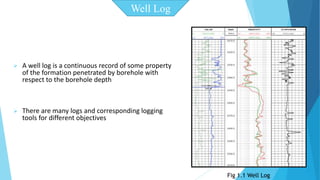
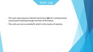
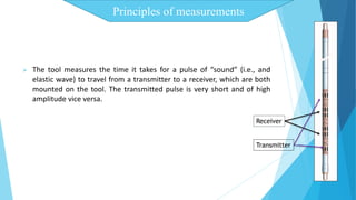
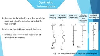
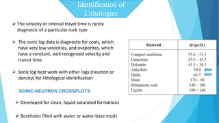
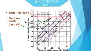
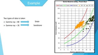
The document discusses the principles and applications of sonic logs in geological technology, detailing various types of tools and their functionality in measuring properties of formations. It explains how sonic logs determine porosity, compaction, overpressure, and assist in stratigraphic correlation, emphasizing their importance in accurately interpreting geological formations. Additionally, it outlines the use of sonic logs for identifying lithologies and the relevance of the Wyllie time average equation in analyzing transit times through different rock types.

1. Presented by
Badal Dutt Mathur
10410007
5th Year Integrated M.tech Geological Technology

2.  A well log is a continuous record of some property
of the formation penetrated by borehole with
respect to the borehole depth
 There are many logs and corresponding logging
tools for different objectives
Well Log
Fig 1.1 Well Log

3. Sonic Log
 The sonic log measures interval transit time (Δt) of a compressional
sound wave traveling through one foot of formation.
 The units are micro seconds/ft, which is the inverse of velocity.

4. Principles of measurements
 The tool measures the time it takes for a pulse of “sound” (i.e., and
elastic wave) to travel from a transmitter to a receiver, which are both
mounted on the tool. The transmitted pulse is very short and of high
amplitude vice versa.
Receiver
Transmitter

5. Working Tools
1.Early Tool
2.Dual Receiver Tool
3.Borehole Compensated Sonic(BHC) Tool

6. Tx
Rx
A
B
C
1. Early tools had one Tx and one Rx.
2. The body of the tool was made from rubber
(low velocity and high attenuation material) to
stop wave travelling preferentially down the
tool to the Rx.
 There was main problems with this tool.
 The measured travel time was always too long.
Δt=A+B+C
Early Tool
Fig 1.2 Early Sonic Tools

7. Rx2
A
B
C
Rx1 D
E
Tx
Dual Receiver Tool
• These tools were designed to overcome the
problems in the early tools.
• They use two receivers a few feet apart, and
measure the difference in times of arrival of
elastic waves at each Receiver from a given pulse
from the Transmitter
• This time is called the sonic interval transit time
(Δt)
 TRx1= A+B+C
 TRx2= A+B+D+E
 Δt=(A+B+D+E)-(A+B+C)
 Δt=D ( If tool is axial in borehole C=E)
Fig 1.3 Dual receiver sonic tools in correct configuration

8. Tx
Rx
Rx
Problem with Dual
 If the tool is tilted in the hole, or the hole size
changes (Fig 3)
 Then C≠E
 The two Rx system fails to work.
Arrangement
C
D
Fig 1.4 Dual receiver sonic tools in incorrect configuration

9. B A
 Automatically compensates for borehole
effects and sonde tilt
 It has two transmitters and four receivers,
arranged in two dual receiver sets, but with
one set inverted
 Each of the transmitters is pulsed
alternately, and Δt values are measured
from alternate pairs of receivers (Fig.1.5)
 These two values of Δt are then averaged
to compensate for tool misalignment
 Δt=A+B/2
Borehole
Compensated Tool
Fig1.5 Borehole compensated sonic tools

10.  Porosity Determination
 Secondary and Fracture Porosity
 Stratigraphic Correlation
 Compaction
 Overpressure
 Synthetic Siesmogram
 Identification of Lithology
Applications

11.  The sonic log is commonly used to calculate the porosity of formations,
however the values from the FDC and CNL logs are superior.
 It is useful in the following ways:
1. As a quality check on the FDC and CNL log determinations.
2. As a robust method in boreholes of variable size (since the sonic log is
relatively insensitive to caving and wash-outs etc.).
3. To calculate secondary porosity in carbonates.
4. To calculate fracture porosity.
Porosity
Determination

12.  The velocity of elastic waves through a given lithology is a function of
porosity
Øsonic = sonic derived porosity in clean formation
Δt = interval transit time of formation
Δtma = interval transit time of the matrix
(sandstone=55.5,limestone=47.6,dolomite=43.5,anhydrite=50)
Δtp = interval transit time of the pore fluid in the well bore
(fresh mud = 189; salt mud = 185)
Unit=microsecond per feet
The Wyllie Time
Average Equation
Fig 1.6 The wave path through porous fluid saturated rocks

13.  Wyllie Time Average Equation is valid only for
 For clean and consolidated sandstones
 Uniformly distributed small pores
 Correction: Observed transit times are greater in uncompacted sands; thus apply
empirical correction factor, Cp
 Фc= Ф/Cp
 Cp=c* Δtsh/100 (Δtsh= Interval transit time for the adjacent shale)
 C=shale compaction coefficient (ranges from 0.8 < c < 1.3)
 Fluid Effect in high porosity formations with high HC saturation.
 Correct by
 OIL: Фcorr= Фc*0.9
 GAS: Фcorr= Фc*0.7
The Wyllie Time
Average Equation

14.  The sonic log is sensitive only to the primary intergranular porosity
 The sonic pulse will follow the fastest path to the receiver and this will
avoid fractures
 Comparing sonic porosity to a global porosity (density log, neutron
log)should indicate zone of fracture.
 Ф2 = (ФN , ФD ) - ФS
Secondary and
Fracture Porosity

15. Fig 1.7 Subtle textural and structural variations in deep sea
turbidite sands shown on the sonic log (after Rider).
 The sonic log is sensitive to small changes in grain
size, texture, mineralogy, carbonate content,
quartz content as well as porosity
 This makes it a very useful log for using for
correlation and facies analysis
Stratigraphic
Correlation

16. Fig 1.8 Uplift and erosion from compaction trends.
Compaction
 As a sediment becomes compacted, the velocity
of elastic waves through it increases
 If one plots the interval transit time on a
logarithmic scale against depth on a linear scale,
a straight line relationship emerges
 Compaction trends are constructed for single
lithologies, comparing the same stratigraphic
interval at different depths
 Compaction is generally accompanied by
diagenetic changes which do not alter after uplift
 Amount of erosion at unconformities or the
amount of uplift from these trends can be
estimated

17. Fig 1.9 An overpressured zone
distinguished from sonic log data.
Overpressure
 An increase in pore pressures is shown on the
sonic log by a drop in sonic velocity or an
increase in sonic travel time
Break in the compaction trend with depth to higher
transit times with no change in lithology
Indicates the top of an
overpressured zone.

18. synthetic
seismogram
acoustic
impedenc
e
reflection
coefficient
reflection
coeffiecient
with
transmission
losses
sonic
 Represents the seismic trace that should be velocity
observed with the seismic method at the
well location
 Improve the picking of seismic horizons
 Improve the accuracy and resolution of
formations of interest
Synthetic
Seismograms
Fig 1.10 The construction of a synthetic seismogram.

19. Identification of
Lithologies
 The velocity or interval travel time is rarely
diagnostic of a particular rock type
 The sonic log data is diagnostic for coals, which
have very low velocities, and evaporites, which
have a constant, well recognized velocity and
transit time
 Sonic log best work with other logs (neutron or
density) for lithological identification
SONIC-NEUTRON CROSSPLOTS
 Developed for clean, liquid-saturated formations
 Boreholes filled with water or water-base muds

20. 110
• Shale - NE region
Field
observation
100
Fracture -
South 90
Gas - NW
80
70
Trona
60
50
40
0 10 20 30
40
Apparent neutron porosity (lspu)
t, Sonic transit time (μs/ft)
Time a
verage
Syivite
Tr
SONIC-NEUTRON
PLOTS

21. Example
Two types of data is taken
 Gamma ray > 80
 Gamma ray < 30
Shale
Sandstone

22.  Serra, O. (1988) Fundamentals of well-log interpretation. 3rd ed. New
York: Elselvier science publishers B.V.: 261-262
 Rider, M. (2002) The geological interpretation of well logs. 2nd ed.
Scotland: Rider French consulting Ltd.: 26-32.
 Neuendorf, et al. (2005) Glossary of Geology. 5th ed. Virginia: American
geological institute: 90, 379, 742.
 Schlumberger (1989) Log interpretation principles/applications.
Schlumberger,Houston, TX
Refrences