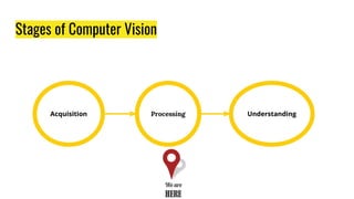
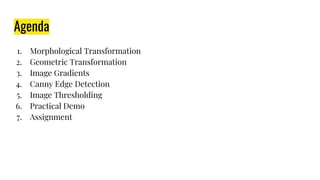
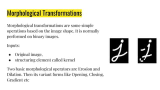
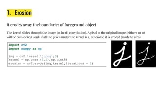
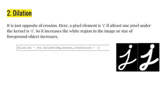
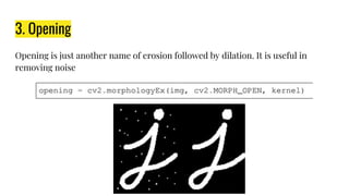
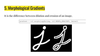
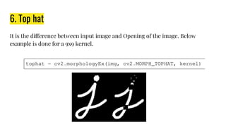
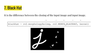
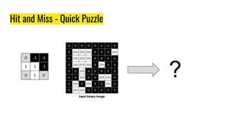
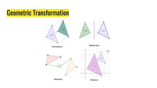
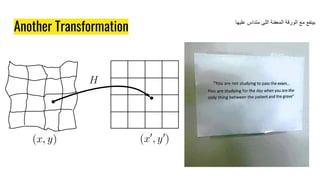
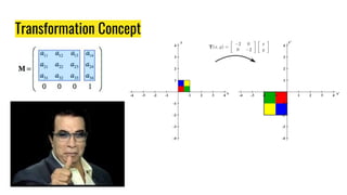
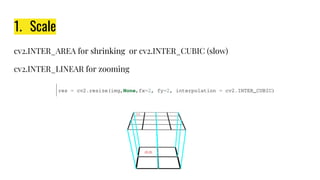
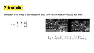
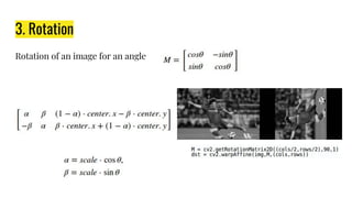
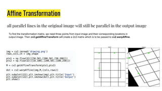
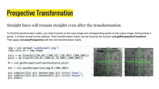
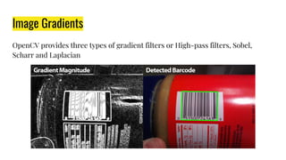
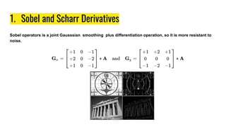
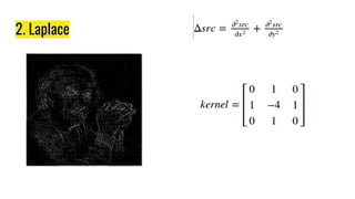
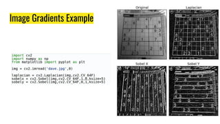
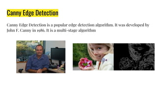
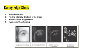
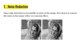
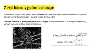
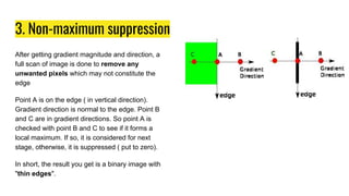
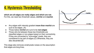
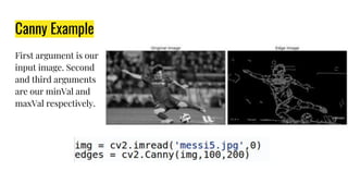
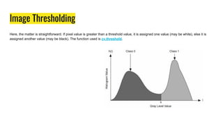
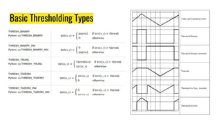
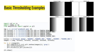
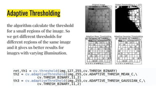
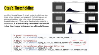
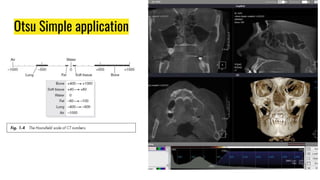
Practical 2 - Digital Image
Processing
Aly Osama
Stages of Computer Vision
Agenda
1. Morphological Transformation
2. Geometric Transformation
3. Image Gradients
4. Canny Edge Detection
5. Image Thresholding
6. Practical Demo
7. Assignment
Morphological
Transformation
Morphological Transformations
Morphological transformations are some simple
operations based on the image shape. It is normally
performed on binary images.
Inputs:
● Original image,
● structuring element called kernel
Two basic morphological operators are Erosion and
Dilation. Then its variant forms like Opening, Closing,
Gradient etc
1. Erosion
it erodes away the boundaries of foreground object.
The kernel slides through the image (as in 2D convolution). A pixel in the original image (either 1 or 0)
will be considered 1 only if all the pixels under the kernel is 1, otherwise it is eroded (made to zero).
2. Dilation
It is just opposite of erosion. Here, a pixel element is ‘1’ if atleast one pixel under
the kernel is ‘1’. So it increases the white region in the image or size of
foreground object increases.
3. Opening
Opening is just another name of erosion followed by dilation. It is useful in
removing noise
4. Closing
Closing is reverse of Opening, Dilation followed by Erosion. It is useful in closing
small holes inside the foreground objects, or small black points on the object.
5. Morphological Gradients
It is the difference between dilation and erosion of an image.
6. Top hat
It is the difference between input image and Opening of the image. Below
example is done for a 9x9 kernel.
7. Black Hat
It is the difference between the closing of the input image and input image.
Structural elements
We manually created a structuring elements in the previous examples but
cv2.getStructuringElement() You just pass the shape and size of the kernel
Hit and Miss Transform - Theory
The Hit-or-Miss transformation is useful to find patterns in binary images. In
particular, it finds those pixels whose neighbourhood matches the shape of a
first structuring element B1 while not matching the shape of a second structuring
element B2
Hit and Miss - Example
B1 B2 B
Hit and Miss - Code
Hit and Miss - Quick Puzzle
?
Geometric Transformation
Another Transformation
‫ﻋﻠﯾﮭﺎ‬ ‫ﻣﺗداس‬ ‫اﻟﻠﻰ‬ ‫اﻟﻣﻌﻔﻧﺔ‬ ‫اﻟورﻗﺔ‬ ‫ﻣﻊ‬ ‫ﺑﯾﻧﻔﻊ‬
Transformation Concept
1. Scale
cv2.INTER_AREA for shrinking or cv2.INTER_CUBIC (slow)
cv2.INTER_LINEAR for zooming
2. Translation
Translation is the shifting of object's location. If you know the shift in (x,y) direction, let it be (tx,ty),
3. Rotation
Rotation of an image for an angle
Affine Transformation
all parallel lines in the original image will still be parallel in the output image
To find the transformation matrix, we need three points from input image and their corresponding locations in
output image. Then cv2.getAffineTransform will create a 2x3 matrix which is to be passed to cv2.warpAffine.
Prospective Transformation
Straight lines will remain straight even after the transformation
To find this transformation matrix, you need 4 points on the input image and corresponding points on the output image. Among these 4
points, 3 of them should not be collinear. Then transformation matrix can be found by the function cv2.getPerspectiveTransform.
Then apply cv2.warpPerspective with this 3x3 transformation matrix.
Image Gradients
Image Gradients
OpenCV provides three types of gradient filters or High-pass filters, Sobel,
Scharr and Laplacian
1. Sobel and Scharr Derivatives
Sobel operators is a joint Gausssian smoothing plus differentiation operation, so it is more resistant to
noise.
2. Laplace
Image Gradients Example
Canny Edge Detection
Canny Edge Detection is a popular edge detection algorithm. It was developed by
John F. Canny in 1986. It is a multi-stage algorithm
Canny Edge Steps
1. Noise Reduction
2. Finding Intensity Gradient of the Image
3. Non-maximum Suppression
4. Hysteresis Thresholding
1. Noise Reduction
Since edge detection is susceptible to noise in the image, first step is to remove
the noise in the image with a 5x5 Gaussian filter.
2. Find Intensity gradients of images
Smoothened image is then filtered with a Sobel kernel in both horizontal and vertical direction to get first
derivative in horizontal direction ( Gx) and vertical direction ( Gy).
Gradient direction is always perpendicular to edges. It is rounded to one of four angles representing
vertical, horizontal and two diagonal directions.
3. Non-maximum suppression
After getting gradient magnitude and direction, a
full scan of image is done to remove any
unwanted pixels which may not constitute the
edge
Point A is on the edge ( in vertical direction).
Gradient direction is normal to the edge. Point B
and C are in gradient directions. So point A is
checked with point B and C to see if it forms a
local maximum. If so, it is considered for next
stage, otherwise, it is suppressed ( put to zero).
In short, the result you get is a binary image with
"thin edges".
4. Hysteresis Thresholding
which are all edges are really edges and which are not.
For this, we need two threshold values, minVal and maxVal.
● Any edges with intensity gradient more than maxVal are
sure to be edges. (A)
● Those below minVal are sure to be non-edges
● Those who lie between these two thresholds are
classified edges or non-edges based on their connectivity.
If they are connected to "sure-edge" pixels, they are
considered to be part of edges.(C) Otherwise, they are
also discarded.(B)
This stage also removes small pixels noises on the assumption
that edges are long lines.
Canny Example
First argument is our
input image. Second
and third arguments
are our minVal and
maxVal respectively.
Image Thresholding
Image Thresholding
Here, the matter is straightforward. If pixel value is greater than a threshold value, it is assigned one value (may be white), else it is
assigned another value (may be black). The function used is cv.threshold.
Basic Thresholding Types
Basic Thresholding Examples
Adaptive Thresholding
the algorithm calculate the threshold
for a small regions of the image. So
we get different thresholds for
different regions of the same image
and it gives us better results for
images with varying illumination.
Otsu’s Thresholding
consider a bimodal image (In simple words, bimodal image is an
image whose histogram has two peaks). For that image, we can
approximately take a value in the middle of those peaks as
threshold value, right ? That is what Otsu binarization does. So in
simple words, it automatically calculates a threshold
value from image histogram for a bimodal image.
Otsu Simple application
Practical Demo
Better Object Tracker Demo
A better Object tracker using
Meanshift and Camshift
Assignment
CSE 101 How to read a Text ?
● Just read it yourself.
● Don’t invent anything not mentioned.
● Don’t be Attef
Assignment 2
● Description: Exercise on Morphological Operations
○ https://goo.gl/sVyLX4
● Points: 5 points
● Team: Individual
● Deliverables:
○ Jupyter (html) notebook to
○ Form Link https://goo.gl/forms/YSzOSpr7QxIlSQht1
● Deadline: 10th March 2018
‫ﺻﻧﺎب‬ ‫ھﯾﻛون‬ ‫ﻛﺎن‬ ‫ﺑس‬ ‫ھو‬ ,‫ﺑﺎﻟﺷﻐل‬ ‫ﻋﻼﻗﺔ‬ ‫ﻣﺎﻟﮭﺎش‬ ‫اﻟﺻورة‬
‫اﺳﮭل‬ ‫ﻟﺣﺎﺟﺔ‬ ‫ﻏﯾرﺗﮫ‬ ‫ﻟﻛن‬ ‫ﺷﺎت‬
Have a question?!
If you have any question
● Facebook
○ You can ask me through Facebook but don’t wait for any
respond before 1 month. “Simply don’t use facebook”
● Office Hours
○ Wednesday 11:30 to 12:30
● Email
○ aly.osama@eng.asu.edu.eg (Response time one day)

Practical Digital Image Processing 2

  • 1.
    Practical 2 -Digital Image Processing Aly Osama
  • 3.
  • 4.
    Agenda 1. Morphological Transformation 2.Geometric Transformation 3. Image Gradients 4. Canny Edge Detection 5. Image Thresholding 6. Practical Demo 7. Assignment
  • 5.
  • 6.
    Morphological Transformations Morphological transformationsare some simple operations based on the image shape. It is normally performed on binary images. Inputs: ● Original image, ● structuring element called kernel Two basic morphological operators are Erosion and Dilation. Then its variant forms like Opening, Closing, Gradient etc
  • 7.
    1. Erosion it erodesaway the boundaries of foreground object. The kernel slides through the image (as in 2D convolution). A pixel in the original image (either 1 or 0) will be considered 1 only if all the pixels under the kernel is 1, otherwise it is eroded (made to zero).
  • 8.
    2. Dilation It isjust opposite of erosion. Here, a pixel element is ‘1’ if atleast one pixel under the kernel is ‘1’. So it increases the white region in the image or size of foreground object increases.
  • 9.
    3. Opening Opening isjust another name of erosion followed by dilation. It is useful in removing noise
  • 10.
    4. Closing Closing isreverse of Opening, Dilation followed by Erosion. It is useful in closing small holes inside the foreground objects, or small black points on the object.
  • 11.
    5. Morphological Gradients Itis the difference between dilation and erosion of an image.
  • 12.
    6. Top hat Itis the difference between input image and Opening of the image. Below example is done for a 9x9 kernel.
  • 13.
    7. Black Hat Itis the difference between the closing of the input image and input image.
  • 14.
    Structural elements We manuallycreated a structuring elements in the previous examples but cv2.getStructuringElement() You just pass the shape and size of the kernel
  • 15.
    Hit and MissTransform - Theory The Hit-or-Miss transformation is useful to find patterns in binary images. In particular, it finds those pixels whose neighbourhood matches the shape of a first structuring element B1 while not matching the shape of a second structuring element B2
  • 16.
    Hit and Miss- Example B1 B2 B
  • 17.
  • 18.
    Hit and Miss- Quick Puzzle ?
  • 19.
  • 20.
  • 21.
    Another Transformation ‫ﻋﻠﯾﮭﺎ‬ ‫ﻣﺗداس‬‫اﻟﻠﻰ‬ ‫اﻟﻣﻌﻔﻧﺔ‬ ‫اﻟورﻗﺔ‬ ‫ﻣﻊ‬ ‫ﺑﯾﻧﻔﻊ‬
  • 22.
  • 23.
    1. Scale cv2.INTER_AREA forshrinking or cv2.INTER_CUBIC (slow) cv2.INTER_LINEAR for zooming
  • 24.
    2. Translation Translation isthe shifting of object's location. If you know the shift in (x,y) direction, let it be (tx,ty),
  • 25.
    3. Rotation Rotation ofan image for an angle
  • 26.
    Affine Transformation all parallellines in the original image will still be parallel in the output image To find the transformation matrix, we need three points from input image and their corresponding locations in output image. Then cv2.getAffineTransform will create a 2x3 matrix which is to be passed to cv2.warpAffine.
  • 27.
    Prospective Transformation Straight lineswill remain straight even after the transformation To find this transformation matrix, you need 4 points on the input image and corresponding points on the output image. Among these 4 points, 3 of them should not be collinear. Then transformation matrix can be found by the function cv2.getPerspectiveTransform. Then apply cv2.warpPerspective with this 3x3 transformation matrix.
  • 28.
  • 29.
    Image Gradients OpenCV providesthree types of gradient filters or High-pass filters, Sobel, Scharr and Laplacian
  • 30.
    1. Sobel andScharr Derivatives Sobel operators is a joint Gausssian smoothing plus differentiation operation, so it is more resistant to noise.
  • 31.
  • 32.
  • 33.
  • 34.
    Canny Edge Detection CannyEdge Detection is a popular edge detection algorithm. It was developed by John F. Canny in 1986. It is a multi-stage algorithm
  • 35.
    Canny Edge Steps 1.Noise Reduction 2. Finding Intensity Gradient of the Image 3. Non-maximum Suppression 4. Hysteresis Thresholding
  • 36.
    1. Noise Reduction Sinceedge detection is susceptible to noise in the image, first step is to remove the noise in the image with a 5x5 Gaussian filter.
  • 37.
    2. Find Intensitygradients of images Smoothened image is then filtered with a Sobel kernel in both horizontal and vertical direction to get first derivative in horizontal direction ( Gx) and vertical direction ( Gy). Gradient direction is always perpendicular to edges. It is rounded to one of four angles representing vertical, horizontal and two diagonal directions.
  • 38.
    3. Non-maximum suppression Aftergetting gradient magnitude and direction, a full scan of image is done to remove any unwanted pixels which may not constitute the edge Point A is on the edge ( in vertical direction). Gradient direction is normal to the edge. Point B and C are in gradient directions. So point A is checked with point B and C to see if it forms a local maximum. If so, it is considered for next stage, otherwise, it is suppressed ( put to zero). In short, the result you get is a binary image with "thin edges".
  • 39.
    4. Hysteresis Thresholding whichare all edges are really edges and which are not. For this, we need two threshold values, minVal and maxVal. ● Any edges with intensity gradient more than maxVal are sure to be edges. (A) ● Those below minVal are sure to be non-edges ● Those who lie between these two thresholds are classified edges or non-edges based on their connectivity. If they are connected to "sure-edge" pixels, they are considered to be part of edges.(C) Otherwise, they are also discarded.(B) This stage also removes small pixels noises on the assumption that edges are long lines.
  • 40.
    Canny Example First argumentis our input image. Second and third arguments are our minVal and maxVal respectively.
  • 41.
  • 42.
    Image Thresholding Here, thematter is straightforward. If pixel value is greater than a threshold value, it is assigned one value (may be white), else it is assigned another value (may be black). The function used is cv.threshold.
  • 43.
  • 44.
  • 45.
    Adaptive Thresholding the algorithmcalculate the threshold for a small regions of the image. So we get different thresholds for different regions of the same image and it gives us better results for images with varying illumination.
  • 46.
    Otsu’s Thresholding consider abimodal image (In simple words, bimodal image is an image whose histogram has two peaks). For that image, we can approximately take a value in the middle of those peaks as threshold value, right ? That is what Otsu binarization does. So in simple words, it automatically calculates a threshold value from image histogram for a bimodal image.
  • 47.
  • 48.
  • 49.
    Better Object TrackerDemo A better Object tracker using Meanshift and Camshift
  • 50.
  • 51.
    CSE 101 Howto read a Text ? ● Just read it yourself. ● Don’t invent anything not mentioned. ● Don’t be Attef
  • 52.
    Assignment 2 ● Description:Exercise on Morphological Operations ○ https://goo.gl/sVyLX4 ● Points: 5 points ● Team: Individual ● Deliverables: ○ Jupyter (html) notebook to ○ Form Link https://goo.gl/forms/YSzOSpr7QxIlSQht1 ● Deadline: 10th March 2018 ‫ﺻﻧﺎب‬ ‫ھﯾﻛون‬ ‫ﻛﺎن‬ ‫ﺑس‬ ‫ھو‬ ,‫ﺑﺎﻟﺷﻐل‬ ‫ﻋﻼﻗﺔ‬ ‫ﻣﺎﻟﮭﺎش‬ ‫اﻟﺻورة‬ ‫اﺳﮭل‬ ‫ﻟﺣﺎﺟﺔ‬ ‫ﻏﯾرﺗﮫ‬ ‫ﻟﻛن‬ ‫ﺷﺎت‬
  • 53.
  • 54.
    If you haveany question ● Facebook ○ You can ask me through Facebook but don’t wait for any respond before 1 month. “Simply don’t use facebook” ● Office Hours ○ Wednesday 11:30 to 12:30 ● Email ○ aly.osama@eng.asu.edu.eg (Response time one day)