This document provides practice exercises for an introduction to research in information studies course. It includes questions on defining statistical terms, computing descriptive statistics like mean, median and mode for sample data, generating frequency distributions and histograms, hypothesis testing, and constructing confidence intervals. The exercises cover topics like measures of central tendency and dispersion, probability distributions, sampling distributions, and both descriptive and inferential statistics.

1. PRACTICE EXERCISES
LIS 397C
Introduction to Research in Information Studies
School of Information
University of Texas at Austin
Dr. Philip Doty
Version 3.5
Copyright Philip Doty, University of Texas at Austin, August 2004 1

2. LIS 397C
Doty
Practice Exercises 3.5
1. Define the following terms and symbols:
n
x∑
x
x
s
s 2
N
µ
σ
σ 2
coefficient of variation (CV)
mode
median
arithmetic mean
range
variance
interquartile range (IQR)
standard deviation
sample
statistic
parameter
frequency distribution
2. A sample of the variable x assumes the following values:
9 11 13 3 7 2 8 9 6 10
Compute:
(a) n
(b) x∑
(c) x
(d) s
(e) s 2
(f) median
(g) mode
(h) range
Copyright Philip Doty, University of Texas at Austin, August 2004 2

3. (i) CV
Copyright Philip Doty, University of Texas at Austin, August 2004 3

4. 3. A sample of the variable x assumes the following values:
57 51 58 52 50 59 57 51 59 56
50 53 54 50 57 51 53 55 52 54
Generate a frequency distribution indicating x, frequency of x, cumulative
frequency of x, relative frequency of x, and cumulative relative frequency
of x.
4. For the frequency distribution in problem 3, compute:
(a) n
(b) x∑
(c) x
(d) s
(e) s 2
(f) median
(g) mode
(h) range
(i) CV
5. Generate a histogram for the data in problem 3.
6. Generate a frequency polygon for the data in problem 3.
7. Define the following terms:
skewness
ordinate
abscissa
central tendency
bimodal
ordered pair
Cartesian plane
stem-and-leaf plot
outlier
reliability
dispersion or variability
negatively skewed
positively skewed
validity
box plot
whiskers
Copyright Philip Doty, University of Texas at Austin, August 2004 4

5. 8. What is the relationship between or among the terms?
(a) sample/population
(b) x /µ
(c) s/σ
(d) variance/standard deviation
(e) n/N
(f) statistic/parameter
(g) mean, median, mode of the normal curve
(h) coefficient of variation/IQR
9. Graph the following sample distributions (histogram and frequency
polygon) using three different pairs of axes.
Distribution 1 Distribution 2 Distribution 3
Score | Frequency Score | Frequency Score | Frequency
25 4 1 25 2 8
26 10 2 31 4 20
27 6 3 40 6 25
28 3 4 44 8 35
29 3 5 51 10 40
30 1 6 19 12 45
53 1 7 10 13 24
85 1 14 20
10. For each of the distributions in problem 9, answer the following questions.
(a) Is the curve of the distribution positively or negatively skewed?
(b) What is n?
(c) Is the mode > median? Compute the answer and also answer it
graphically, i.e., label the position of the mode and the median on
the curve.
(d) Is the mean > mode? Compute the answer and also answer it
graphically as in part (c) of this question.
(e) What is the variance of the distribution?
(f) What is the standard deviation of the distribution?
(g) What is the range of the distribution?
(h) What is the coefficient of variation of the distribution?
(i) Which measure of central tendency, mode, median, or (arithmetic)
mean, is the fairest and clearest description of the distribution?
Copyright Philip Doty, University of Texas at Austin, August 2004 5

6. Why?
Copyright Philip Doty, University of Texas at Austin, August 2004 6

7. 11. Define:
error model
quartile
percentile
Q 1
Q 2
Q 3
freq (x)
cf (x)
rel freq (x)
cum rel freq (x)
PR
z-scores
χ
deviation score
s of z-scores
x of z-scores
x∑
centile
Interquartile Range (IQR)
non-response bias
self-selection
12. Define the relationship(s) between or among the terms:
Q 2/median
median/N or n
z-score/raw score
z-score/deviation score/standard deviation
Q 1/ Q 2/ Q 3
z-score/ χ/s or σ
median/fifth centile
cf (x)/freq (x)/PR
Literary Digest poll/bias
13. The observations of the values of variable x can be summarized in the
population frequency distribution below.
x freq (x)
9 3
8 9
6 5
Copyright Philip Doty, University of Texas at Austin, August 2004 7

8. 3 2
2 6
Copyright Philip Doty, University of Texas at Austin, August 2004 8

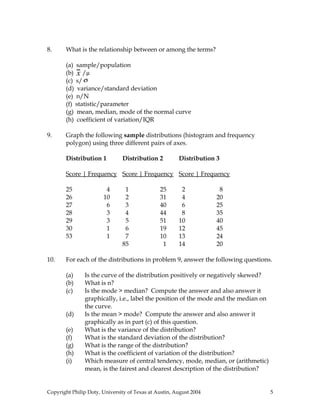
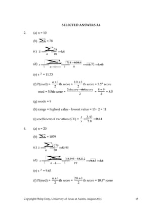
9. For this distribution of x, calculate:
(a) Cumulative frequency, relative frequency, and cumulative relative
frequency for each value
(b) N
(c) the range
(d) median
(e) mode
(f) µ
(g) σ
(h) Q 1, Q 2, and Q 3
(i) CV (coefficient of variation)
(j) IQR
(k) the percentile rank of x = 8, x = 2, x = 3
(l) z-scores for x = 6, x = 8, x = 2, x = 3, x = 9
14. Generate a box plot for the data in problem 13.
15. Generate a box plot for the data in problem 3.
16. For a normally distributed distribution of variable x, where µ = 50 and σ
= 2.5 [ND (50, 2.5)], calculate:
(a) the percentile rank of x = 45
(b) the z-score of x = 52.6
(c) the percentile rank of x = 58
(d) the 29.12th percentile
(e) the 89.74th percentile
(f) the z-score of x = 45
(g) the percentile rank of x = 49
17. Define:
α
sampling distribution
Central Limit Theorem
Standard Error (SE)
ND(µ, σ)
decile
descriptive statistics
inferential statistics
effect size
confidence interval (C.I.) on µ
Copyright Philip Doty, University of Texas at Austin, August 2004 9

10. Student's t
degrees of freedom (df)
random sampling
stratified random sample
Copyright Philip Doty, University of Texas at Austin, August 2004 10

11. 18. Define the relationship(s) between or among the terms:
E( x )/µ
α/df/t
Central Limit Theorem/C.I. on µ
α/C.I. on µ when σ is known
α/C.I. on µ when σ is not known
z/confidence interval on µ
t/C.I. on µ
t/z
19. The following values indicate the number of microcomputer applications
available to a sample of 10 computer users.
2, 5, 9, 5, 3, 6, 6, 3, 1, 13
For the population from which the sample was drawn, µ = 4.1 and
σ = 2.93.
Calculate:
a. The expected value of the mean of the sampling distribution of means
b. The standard deviation of the sampling distribution of means.
20. From previous research, we know that the standard deviation of the ages
of public library users is 3.9 years. If the "average" age of a sample of 90
public library users is 20.3 years, construct:
a. a 95% C.I. around µ
b. a 90% C.I. around µ
c. a 99% C.I. around µ.
What does a 95% interval around µ mean?
What is our best estimate of µ?
21. The sample size in problem 20 was increased to 145, while the "average"
age of the sample remained at 20.3 years. Construct three confidence
intervals around µ with the same levels of confidence as in Question 20.
22. Determine t for a C.I. of 95% around µ when n equals 20, 9, ∞ , and 1.
Copyright Philip Doty, University of Texas at Austin, August 2004 11

12. 23. Determine t on the same values of n (20, 9, ∞ , and 1) as in Question 22,
but for a C.I. of 99% around µ. Should this new interval be narrower or
wider than a 95% confidence interval on µ? Why? Answer the question
both conceptually and algebraically.
24. The following frequency distribution gives the values for variable x in a
sample drawn from a larger population.
x freq(x)
43 6
42 11
39 3
36 7
35 7
34 15
Calculate:
(a) x
(b) s
(c) SEµ = σx
(d) E( x )
(e) Q 1 , Q 2, and Q 3
(f) mode
(g) CV
(h) IQR
(i) a 95% C.I. on µ
(j) the width of the confidence interval in part (i)
(k) a 99% C.I. on µ
(l) the width of the confidence interval in part (k)
(m) PR (percentile rank) of x = 42
(n) our best estimates of µ and σ from the data.
25. Generate a box plot for the data in problem 24.
26. Construct a stem-and-leaf plot for the following data set; indicate Q 1, Q 2
, and Q 3 on the plot; and generate the six-figure summary. Be sure that
you are able to identify the stems and the leaves and to identify their units
of measurement.
The heights of members of an extended family were measured in inches.
The observations were: 62, 48, 56, 37, 37, 26, 74, 66, 29, 49, 72, 77, 69, 62,
Copyright Philip Doty, University of Texas at Austin, August 2004 12

13. and 64.
Copyright Philip Doty, University of Texas at Austin, August 2004 13

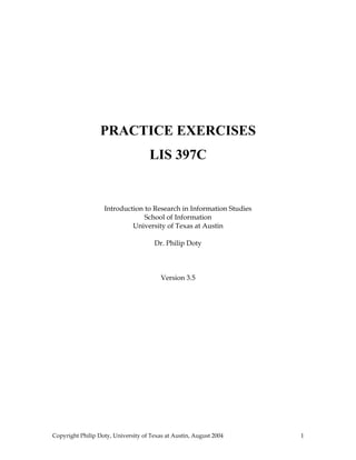
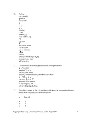
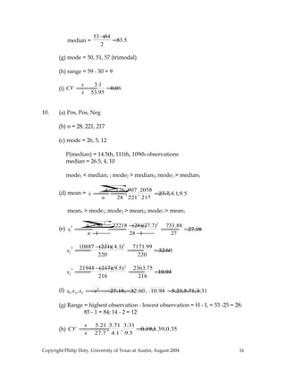
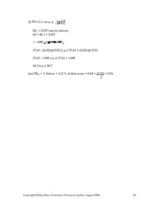
14. 27. H 0: There is no relationship between computer expertise and minutes
spent doing known-item searches in an OPAC at α = 0.10.
Should we reject the H0 given the following data? Remember that the
acceptable error rate is 0.10.
TIME (MINS)
EXPERTISE ≤ 5 > 5, ≤ 10 > 10
Novice 14 20 19
Intermediate 15 16 9
Expert 22 11 2
28. Answer Question 27 at an acceptable error rate of 0.05.
29. Define:
statistical hypothesis
Ho
H1
p
Type I error
Type II error
χ2
nonparametric
contingency table
statistically significant
E (expected value) in χ2
O (observed value) in χ2
30. Discuss the relationship(s) between or among the terms:
α/p
df/R/C [in χ2
situation]
Ho / H1
χ2
/α/df
α/Type I error
E/O/ χ2
Type I/Type II error
Copyright Philip Doty, University of Texas at Austin, August 2004 14

15. SELECTED ANSWERS 3.4
2. (a) n = 10
(b) x∑= 78
(c) x =
x∑
n
=
78
10
=7.8
(d) s =
x2
∑−nx2
n −1
=
714 −608.4
9
=11.73 =3.43
(e) s 2
= 11.73
(f) P(med) =
n +1
2
th score =
10 +1
2
th score = 5.5th
score
med = 5.5th score =
5thscore +6thscore
2
=
8 + 9
2
= 8.5
(g) mode = 9
(h) range = highest value - lowest value = 13 - 2 = 11
(i) coefficient of variation (CV) =
s
x
=
3.43
7.8
=0.44
4. (a) n = 20
(b) x∑= 1079
(c) x =
x∑
n
=
1079
20
=53.95
(d) s =
x 2
∑−nx 2
n −1
=
58395−58212
19
=9.63 =3.1
(e) s 2
= 9.63
(f) P(med) =
n +1
2
th score =
20 +1
2
th score = 10.5th
score
Copyright Philip Doty, University of Texas at Austin, August 2004 15

16. median =
53 +54
2
=53.5
(g) mode = 50, 51, 57 (trimodal)
(h) range = 59 - 50 = 9
(i) CV =
s
x
=
3.1
53.95
=0.06
10. (a) Pos, Pos, Neg
(b) n = 28, 221, 217
(c) mode = 26, 5, 12
P(median) = 14.5th, 111th, 109th observations
median = 26.5, 4, 10
mode1 < median1 ; mode2 > median2; mode3 > median3
(d) mean = x =
x∑
n
=
776
28
;
907
221
;
2058
217
=27.7,4.1,9.5
mean1 > mode1; mode2 > mean2; mode3 > mean3
(e) s1
2
=
x2
∑−nx 2
n −1
=
22218 −(28)(27.7)2
28 −1
=
733.88
27
=27.18
s2
2
=
10887 −(221)(4.1)2
220
=
7171.99
220
=32.60
s3
2
=
21948 −(217)(9.5)2
216
=
2363.75
216
=10.94
(f) s1,s2,s3 =s2
=27.18, 32.60, 10.94 =5.21,5.71,3.31
(g) Range = highest observation - lowest observation = H - L = 53 -25 = 28;
85 - 1 = 84; 14 - 2 = 12
(h) CV =
s
x
=
5.21
27.7
,
5.71
4.1
,
3.31
9.5
=0.19,1.39,0.35
Copyright Philip Doty, University of Texas at Austin, August 2004 16

17. 13. (a) x freq x cum freq x rel freq x cum rel freq x
9 3 25 0.12 1.00
8 9 22 0.36 0.88
6 5 13 0.20 0.52
3 2 8 0.08 0.32
2 6 6 0.24 0.24
25 1.00
(b) N = 25
(c) Range = H - L = 9 - 2 = 7
(d) P(median) = N + 1 th position = 13th observation; median = 6
2
(e) mode = 8
(f) µ=
x∑
N
=
147
25
=5.88
(g) σ=
x 2
∑−Nµ2
N
=
1041−(25)(5.88)2
25
=
174.64
25
=7.07 =2.66
(h) P(Q2) = 13th observation; Q2 = 6
P(Q1) =
1+↓P(Q2 )
2
=
1+13
2
= 7th observation from the beginning; Q1=
3
P(Q3 ) =
1+↓P(Q2)
2
=
1+13
2
= 7th observation from the end; Q3= 8
(i) CV =
σ
µ
=
2.66
5.88
=0.45
(j) IQR = Q3 - Q1 = 8 - 3 = 5
(k) PR = % lower + 1/2 % of that score
PR(8) = 0.52 + (0.36) = 0.70
2
Copyright Philip Doty, University of Texas at Austin, August 2004 17

18. PR(2) = 0 + (0.24) = 0.12
2
PR(3) = 0.24 + (0.08) = 0.28
2
Copyright Philip Doty, University of Texas at Austin, August 2004 18

19. (l) z =
x −µ
σ
(for populations)
z6 =
x −µ
σ
=
6 −5.88
2.66
=0.05;z8 =
8 −5.88
2.66
=0.80;z2 =
2 −5.88
2.66
=−1.46
z3 =
3−5.88
2.66
=−1.08;z9 =
9 −5.88
2.66
=1.17
16. ND(50, 2.5)
(a) PR(45); z45 =
x −µ
σ=
45 −50
2.5
=−2.00 ⇒−0.4772
0.5000 - 0.4772 = 0.0228, 2.28%, 2.28th percentile
(b) z52.6 =
52.6 −50
2.5
=1.04
(c) PR(58); z58 =
58 −50
2.5
=3.2 ⇒0.4993
0.5000 + 0.4993 = 0.9993, 99.93%, 99.93rd percentile
(d) find the 29.12th percentile
0.5000 - 0.2912 = 0.2088 ⇒z = - 0.55
−0.55 =
x −50
2.5
x −50 =−1.375
x =48.63
(e) find the 89.74th percentile
0.8974 - 0.5000 = 0.3974 ⇒z = 1.27
z =1.27 =
x −50
2.5
x =53.175
(f) z45 =
45 −50
2.5
=−2.00
Copyright Philip Doty, University of Texas at Austin, August 2004 19

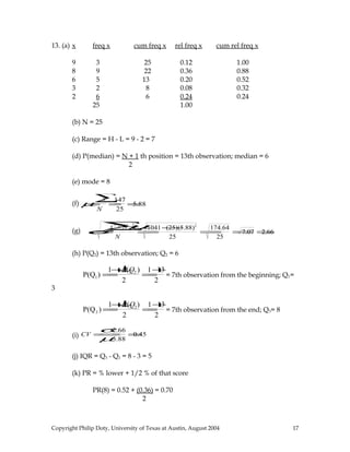
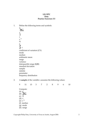
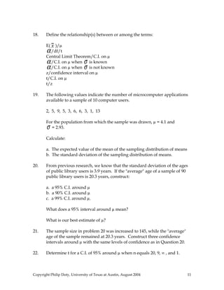
20. (g) PR(49); z49 =
49 −50
2.5
=
−1
2.5
=−0.4 ⇒−0.1554
0.5000 – 0.1554 =0.3446, 34.46%, 34.46th
percentile
19. 2, 5, 9, 5, 3, 6, 6, 3, 1, 13
(a) E(x) =µ=4.1
(b) SEµ=σx =
σ
n
=
2.93
10
=0.93
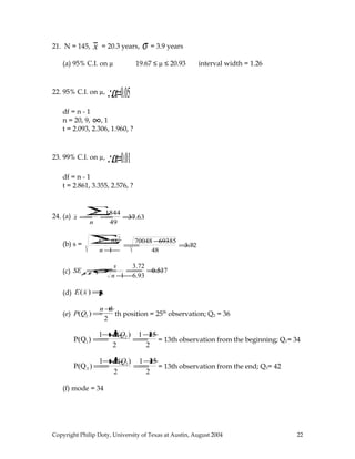
20. σ=3.9 years, n = 90, x =20.3 years
(a) 95% C.I. on µ x −zSEµ≤µ≤x +zSEµ
SEµ=σx =
σ
n
=
3.9
90
=0.41
z95% = 1.96 [Remember that
0.95
2
=0.4750⇒1.96 =z]
x −zSEµ≤µ≤x +zSEµ
20.3 - (1.96)(0.41) ≤ µ ≤ 20.3 + (1.96)(0.41)
19.5 ≤ µ ≤ 21.1 interval width = 1.6
(b) 90% C.I. on µ z90%= 1.65
x −zSEµ≤µ≤x +zSEµ
20.3 - (1.65)(0.41) ≤ µ ≤ 20.3 + (1.65)(0.41)
19.62 ≤ µ ≤ 20.98 interval width = 1.36
(c) 99% C.I. on µ z99%= 2.58
x −zSEµ≤µ≤x +zSEµ
20.3 - (2.58)(0.41) ≤ µ ≤ 20.3 + (2.58)(0.41)
19.25 ≤ µ ≤ 21.35 interval width = 2.1
Copyright Philip Doty, University of Texas at Austin, August 2004 20

21. Our best estimate of µ is x , 20.3 years
Copyright Philip Doty, University of Texas at Austin, August 2004 21

22. 21. N = 145, x = 20.3 years, σ = 3.9 years
(a) 95% C.I. on µ 19.67 ≤ µ ≤ 20.93 interval width = 1.26
22. 95% C.I. on µ, ∴α=0.05
df = n - 1
n = 20, 9, ∞, 1
t = 2.093, 2.306, 1.960, ?
23. 99% C.I. on µ, ∴α=0.01
df = n - 1
t = 2.861, 3.355, 2.576, ?
24. (a) x =
x∑
n
=
1844
49
=37.63
(b) s =
x2
∑−nx2
n −1
=
70048 −69385
48
=3.72
(c) SEµ=σx =
s
n −1
=
3.72
6.93
=0.537
(d) E(x ) =µ
(e) P(Q2 ) =
n +1
2
th position = 25th
observation; Q2 = 36
P(Q1) =
1+↓P(Q2 )
2
=
1+25
2
= 13th observation from the beginning; Q1= 34
P(Q3 ) =
1+↓P(Q2)
2
=
1+25
2
= 13th observation from the end; Q3= 42
(f) mode = 34
Copyright Philip Doty, University of Texas at Austin, August 2004 22

23. (g) CV =
s
x
=
3.72
37.63
=0.10
(h) IQR = Q3 – Q1 = 42 - 34 = 8
Copyright Philip Doty, University of Texas at Austin, August 2004 23

24. (i) 95% C.I. on µ, µ, ∴α=0.05
SEµ = 0.537 (see (c) above)
df = 48, t = 2.021
x −zSEµ≤µ≤x +zSEµ
37.63 - (2.021)(0.537) ≤ µ ≤ 37.63 + (2.021)(0.537)
37.63 - 1.085 ≤ µ ≤ 37.63 + 1.085
36.5 ≤ µ ≤ 38.7
(m) PR42 = % below + 1/2 % of that score = 0.65 + (0.22) = 0.76
2
Copyright Philip Doty, University of Texas at Austin, August 2004 24

25. 27.
TIME (MINS)
≤5 >5, ≤10 >10
EXPERTISE
Novice 14 (21.12) 20 (19.46) 19 (12.42) 53
Intermediate 15 (15.94) 16 (14.69) 9 (9.38) 40
Expert 22 (13.95) 11 (12.85) 2 (8.20) 35
51 47 30 128
χ2
=
(O −E)2
E
E =
RxC
n
χ2
=
(14 −21.12)2
21.12
+
(15 −15.94)2
15.94
+
(22 −13.95)2
13.95
+
(20 −19.46)2
19.46
+
(16 −14.69)2
14.69
+
(11−12.85)2
12.85
+
(19 −12.42)2
12.42
+
(9 −9.38)2
9.38
+
(2 −8.20)2
8.20
χ2
= 2.40 + 0.06 + 4.65 + 0.01 + 0.12 + 0.27 + 3.49 + 0.02 + 4.69 = 15.71
df = (R - 1)(C - 1) = 2 x 2 = 4
χ2
(4, 0.10) = 7.78
15.71 > 7.78, reject H0
28. χ2
(4, 0.05) = 9.49
15.71 > 9.49, reject H0
Copyright Philip Doty, University of Texas at Austin, August 2004 25