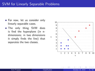
This document provides an overview of Support Vector Machines (SVMs). It discusses how SVMs find the optimal separating hyperplane between two classes that maximizes the margin between them. It describes how SVMs can handle non-linearly separable data using kernels to project the data into higher dimensions where it may be linearly separable. The document also discusses multi-class classification approaches for SVMs and how they can be used for anomaly detection.


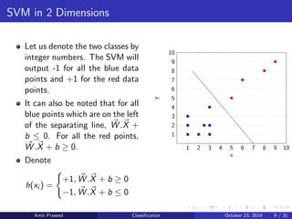
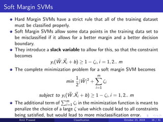
![SVM in 2 Dimensions
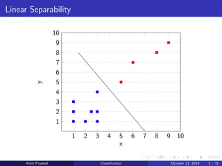
In two dimensions, the problem reduces to finding the optimal line sep-
arating the two data classes. The conditions for the optimal hyperplane
still hold in two dimensions.
Let the line we have to find be y = ax + b.
y = ax + b
ax − y + b = 0
Let X = [x y] and W = [a − 1], then the equation for the line
becomes
W .X + b = 0
which incidentally is the equation for a hyperplane as well, when gen-
eralized to n dimensions. Here W is a vector perpendicular to the
plane.
Amit Praseed Classification October 23, 2019 8 / 31](https://image.slidesharecdn.com/svm-200407155627/85/Support-Vector-Machines-SVM-8-320.jpg)


![SVM[Support vector Machine] Machine learning](https://cdn.slidesharecdn.com/ss_thumbnails/svm-250403184638-1cd9afdb-thumbnail.jpg?width=640&height=640&fit=bounds)


![[ML]-SVM2.ppt.pdf](https://cdn.slidesharecdn.com/ss_thumbnails/ml-svm2-230916145832-2580c8e3-thumbnail.jpg?width=640&height=640&fit=bounds)