Downloaded 67 times


![CHAPTER 15 Environmental Forecasting
Present
Time - Future
Figure 15.3 Possible trajectories of population change.
cent). If the annual growth rate, r, is expressed as a fraction (such as 0.02), a general
expression for the total population, after t years is
P = Po (1 + r)' [15.1]
where Pu is the initial population at the time t = 0.
This equation has the identical form as the compound annual interest equation
used in engineering economics to calculate monetary growth (see Chapter 13j. The key
characteristic of this equation is a nonlinear increase in the total quantity over time (be
it population, money, or any other quantity that grows at a constant annual rate). Fig-
ure 15.4 illustrates thls trend for three different rates of annual population growth. The
higher the annual growth rate, the more dramatic the rise in population over time.
0
0 10 20 30 40 50
Time (years)
Figure 15.4 Population increase for three annual growth rates based on a
compound annual growth model.](https://image.slidesharecdn.com/populationmodels-111221223843-phpapp01/85/population-models-pdf-4-320.jpg)


![PART 4 Topics in Environmental Policy Analysis
assumed to change over time in the middle series Census Bureau projection. Differ-
ent assumptions produced the higher and lower population projections.
Figure 15.8(c) shows the 2050 population distribution resulting from the middle
series projections. Note that the profile is much more uniform than the 1999 profile in
Figure 15.7(a). These projections imply a higher percentage of older people in the pop-
ulation than today: In the oldest groups the population over 80 will have roughly tripled.
These results have important implications for public policy and the economy. For exam-
ple, demand is likely to increase for health care services (as opposed to schools) and a
smaller percentage of the population will be in the workforce. At the same time more
1,200 -
----- Low series
- - - High series /
/
/
/
/
/
Actual Forecast 0/
0
Year
(a)
Year
(b)
Figure 15.8 U.S. population projections to 2050, showing [a] the low, middle, and high
estimates of the U.S. Census Bureau, (b) key assumptions behind the middle
(best estimate) projection, and [c) the best-estimate age distribution in 2050.
(Source: Based on USDOC, 1999b and 1999c)](https://image.slidesharecdn.com/populationmodels-111221223843-phpapp01/85/population-models-pdf-15-320.jpg)


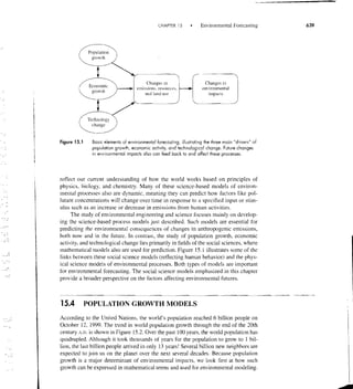
The document discusses models for forecasting population growth and their implications for environmental impacts. It introduces the concept of exponential and logistic growth models. - Exponential growth assumes a constant growth rate leading to ever-increasing population over time. Logistic growth incorporates the finite carrying capacity of the environment, causing population growth to level off as it approaches this limit. - Logistic growth produces an S-shaped curve, initially exponential but then slowing to reach an equilibrium population equal to the environment's carrying capacity. This model more realistically represents constraints on indefinite growth.


![Week 5 [compatibility mode]](https://cdn.slidesharecdn.com/ss_thumbnails/week5compatibilitymode-130213165351-phpapp01-thumbnail.jpg?width=640&height=640&fit=bounds)