![96 Chapter II: Observables and States in Tensor Products of Hilbert Spaces
Exercise 15.11: Let Ᏼn = L2 (
n , Ᏺn , n ), n = 1, 2, . . . , Ᏼ = L2 (
, Ᏺ, )
where (
n , Ᏺn , n ) is a probability space for each n and (
, Ᏺ, ) = 51 1 (
n ,
n=
Ᏺn , n ) is the product probability space. Then Ᏼ is the countable tensor product
of the sequence fᏴn g with respect to the stabilising sequence fn g where n is
the constant function 1 in
n for each n. This may be used to construct examples
where different stabilising sequences may lead to different countable tensor prod-
ucts. (Hint: If and are two distinct probability measures such that then
2 2 1 1 1 and 2 2 1 1 1 are singular with respect to each other.)
Exerecise 15.12: Let Ᏼ = L2 ([0, 1], h) be the Hilbert space defined in Section 2
where is the Lebesgue measure in [0, 1]. Then any continuous map f : [0, 1] ! Ᏼ
is an element of Ᏼ. For any such continuous map f define the element en (f ) in
( 8 ރh)
n by
en (f ) =
n=1 f1 8 n0 21 f ( j )g.
j
n
Then
lim hen (f ), en (g )i = exphf , g i.
n !1
Exercise 15.13: Let Ᏼ1 , Ᏼ2 be Hilbert spaces and let ff1 , f2 , . . .g be an or-
thonormal basis in Ᏼ2 . Then there exists a unitary isomorphism U : Ᏼ1
Ᏼ2 !
Ᏼ1 8 Ᏼ1 8 1 1 1 satisfying Uu
v = 8i hfi , v iu for all u 2 Ᏼ1 , v 2 Ᏼ2 .
Exercise 15.14: Let L2 (, h) be as defined in Section 2. Then there exists a unique
unitary isomorphism U : L2 ()
h ! L2 (, h) satisfying (Uf
u)(! ) = f (! )u.
Exercise 15.15: Let Ᏼ be a Hilbert space and let I2 (Ᏼ) be the Hilbert space of
3
all Hilbert-Schmidt operators in Ᏼ with scalar product hT1 , T2 i = tr T1 T2 . For any
fixed conjugation J there exists a unique unitary isomorphism U : Ᏼ
Ᏼ ! I2 (Ᏼ)
satisfying Uu
v = juihJv j for all u, v in Ᏼ. (See Section 9.)
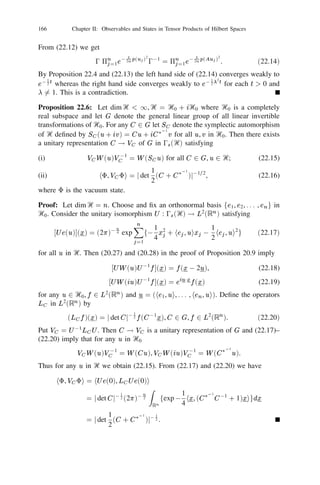
Example 15.16: [20] Let H be any selfadjoint operator in a Hilbert space Ᏼ
with pure point spectrum 6(H ) = S . Then S is a finite or countable subset of
.ޒDenote by G the countable additive group generated by S and endowed with
~
the discrete topology. Let G be its compact character group with the normalised
Haar measure. For any bounded operator X on Ᏼ and 2 G define the bounded
operator Z
X = ()(H )X(H )d.
~
G
Let , 2 S , u, v 2 Ᏼ, Hu = u, Hv = v. Then
Z
hu, X v i = f ( 0 0 )dghu, Xvi.
~
G
Hence hu, Xvi = 0 ,
hu, X v i =
if
0 if 6= 0 .](https://image.slidesharecdn.com/anintroductiontoquantumstochasticcalculus-130327234248-phpapp01/85/An-introduction-to-quantum-stochastic-calculus-20-320.jpg)
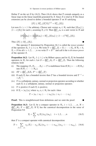
![16 Operators in tensor products of Hilbert spaces 97
Thus, for any non-zero bounded operator X
there exists a 2 S0S =
S X
f 0 j , 2 g such that 6= 0 and on the linear manifold D generated
by all the eigenvectors of H
[H , [H , X ]] = 2 X ,
Xu = X0u +
X (X0 + X )u , u 2 D.
0
2S0S
IfX X X
is selfadjoint ( )3 = 0 and X
is a “superposition” of bounded “har-
X X X S S
monic” observables 0 , f 0 + j 2 0 , 0g with respect to . (See H
XY
tr X 3 Y = tr X0 Y0 +
3
X
Example 6.2.) Whenever , are Hilbert-Schmidt operators
tr X Y
3
2S0S
X (X + X
0
and
X = X0 + 0 )
2S0S
0
converges in Hilbert-Schmidt norm (i.e., the norm in I2 (Ᏼ)). See Example 6.2.
Notes
The presentation here is based on the notes of Parthasarathy and Schmidt [99].
Proposition 15.1 is known as Schur’s Lemma. Proposition 15.4 and Exercise 15.6
constitute what may be called a probability theorist’s translation of the famous
Gelfand-Neumark-Segal or G.N.S. Theorem. Its origin may be traced back to the
theory of second order stationary stochastic processes developed by A.N. Kol-
mogorov, N. Wiener, A.I. Khinchine and K. Karhunen [31]. Proposition 7.2, 15.4
and 19.4 more or less constitute the basic principles around which the fabric of
our exposition in this volume is woven.
e
n
h
It is an interesting idea of Journ´ and Meyer [88] that (
) 8 ރin Exercise
e f
15.12 may be looked upon as a toy Fock space where n ( ) may be imagined as
a toy exponential or coherent vector which in the limit becomes the boson Fock
L h ef
space 0( 2 [0, 1]
) where ( ) is the true exponential or coherent vector. See
Exercise 29.12, 29.13, Parthasarathy [107], Lindsay and Parthasarathy [78].
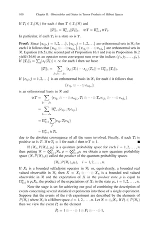
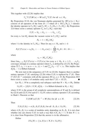
16 Operators in tensor products of Hilbert spaces
n N
We shall now define tensor products of operators. To begin with let Ᏼi be a finite
m i
dimensional Hilbert space of dimension i , = 1, 2, . . . , and Ᏼ = i=1 Ᏼi .
n
T j m
Suppose i is a selfadjoint operator in Ᏼi with eigenvalues f ij , 1 i g
e j m
and corresponding orthnormal set of eigenvectors f ij , 1 i g so that
Tieij = ij eij , 1 j mi, i = 1, 2, . . . , n.
Using Exercise 15.8 define a selfadjoint operator T on Ᏼ by putting
On On
T eiji = 5n=1iji eiji , 1 ji mi
i
i=1 i=1](https://image.slidesharecdn.com/anintroductiontoquantumstochasticcalculus-130327234248-phpapp01/85/An-introduction-to-quantum-stochastic-calculus-21-320.jpg)
![104 Chapter II: Observables and States in Tensor Products of Hilbert Spaces
Exercise 16.11: Let fᏴn , n 0g be a sequence of Hilbert spaces and fn , n 1g
be unit vectors, n 2 Ᏼn . Define Ᏼ[n+1 = Ᏼn+1
Ᏼn+2
1 1 1 with respect to
the stabilising sequence n+1 , n+2 , . . . and Ᏼn] = Ᏼ0
Ᏼ1
1 1 1
Ᏼn . In the
Hilbert space
~
Ᏼ = Ᏼ0
Ᏼ[1 = Ᏼn ]
Ᏼ[n+1 , n = 1, 2, . . .
consider the increasing sequence of *-algebras
= fX
1 n 1 jX 2 B(Ᏼn )g, n = 0, 1, 2 . . .
Bn] [ + ]
Define Bn = B (Ᏼn ) and 1n to be the identity in Bn . There exists a unique linear
] ]
map ޅn : B1 ! Bn satisfying
] ]
hu, ޅn (X )v i = hu
n 1 , Xv
n 1 i for all u, v 2 Ᏼn , X 2 B1
] [ + [ + ]
[ + +
~
where n 1 = n 1
n 2
1 1 1 and B1 = B (Ᏼ). Indeed,
+
ޅn (X ) = ޅn n (X )
1 n 1 .
] j [ +1 ih [ +1 j [ +
The maps fޅn] gn0 satisfy the following properties:
(i) ޅn] 1 = 1, ޅn] X 3 = (ޅn] X )3 , kޅn] X k kX k;
(ii) ޅn] AXB = Aޅn] (X )B whenever A, B 2 Bn] ;
ޅm] ޅn] = ޅn] ޅm] = ޅm] whenever m n;
(iii)
(iv)
P 1i,j k Yi ޅn] (Xi Xj )Yj 0 for all Yi 2 Bn] ,
3 3
Xi 2 B . In particular
1
ޅn] X 0 whenever X 0;
(v) s.limn!1 ޅn] X = X for all X in B1 .
Exercise 16.12: (i) In the notations of Exercise 16.11 a sequence fXn g in B1
is said to be adapted if Xn 2 Bn] for every n. It is called a martingale if
ޅn01] Xn = Xn 01 for all n1
Suppose A = fAn gn 1 is any sequence of operators where
An 2 B(Ᏼn ), hn , An n i = 0, n = 1, 2, . . .
~
Define
An = 1n
An
1[n+1 ,
01]
Mn (A) = A + A + 1 1 1 + A if n = 0,
0
~1 ~2 ~n if n 1.
Then fMn (A)gn0 is a martingale. For any two sequences A, B of operators
where An , Bn 2 B (Ᏼn ), hn , An n i = hn , Bn n i = 0 for each n
ޅm] fMn (A) 0 Mm (A)g3 fMn (B ) 0 Mm (B )g
Xn
= hAj j , Bj j i for all n m 0.
j =m+1](https://image.slidesharecdn.com/anintroductiontoquantumstochasticcalculus-130327234248-phpapp01/85/An-introduction-to-quantum-stochastic-calculus-28-320.jpg)
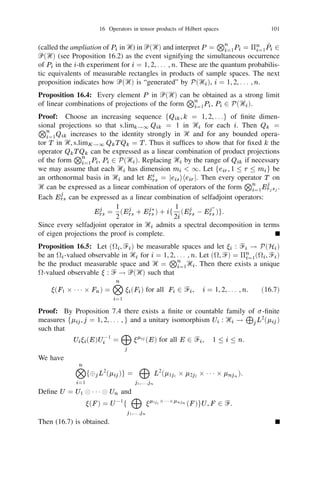
![17 Symmetric and antisymmetric tensor products 105
(ii) For any sequence E = (E1 , E2 , . . .) of operators such that
En 2 Bn01 , n = 1, 2, . . .
]
define 0
In (A, E ) = Pn EnfMn(A) 0 Mn0 (A)g
1 1
if
if
n = 0,
n 1.
Then fIn (A, E )gn0 is a martingale. Furthermore
ޅn01] In (A, E )3 In (B , F ) = In01 (A, E )3 In01 (B , F )
3
+ hAn n , Bn n iEn Fn
for all n 1.
Exercise 16.13: For any selfadjoint operator X in the Hilbert space Ᏼ define
the operator S (X ) in
2ރᏴ by S (X ) = (1
1) exp[i2
X ] where j ,
1 j 3 are the Pauli spin matrices. Then S (X ) = S (X )01 = S (X )3 and
2 [S (X ) + S (0X )] = 1
cos X . Thus S (X ) and S (0X ) are spin observables
1
with two-point spectrum f01, 1g but their average can have arbitrary spectrum in
the interval [01, 1]. (See also Exercise 4.4, 13.11.)
Notes
The role of tensor products of Hilbert spaces and operators in the construction of
observables concerning multiple quantum systems is explained in Mackey [84].
For a discussion of conditional expectation in non-commutative probability theory,
see Accardi and Cecchini [4]. Exercise 16.13 arose from discussions with B.V. R.
Bhat.
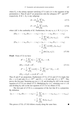
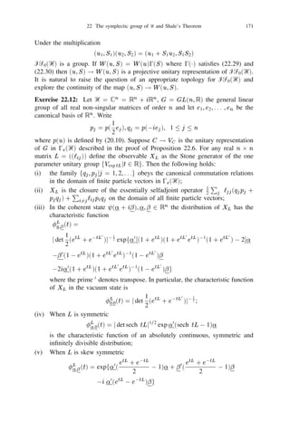
17 Symmetric and antisymmetric tensor products
There is a special feature of quantum mechanics which necessitates the introduction
of symmetric and antisymmetric tensor products of Hilbert spaces. Suppose that
a physical system consists of n identical particles which are indistinguishable
from one another. A transition may occur in the system resulting in merely the
interchange of particles regarding some physical characteristic (like position for
example) and it may not be possible to detect such a change by any observable
means. Suppose the statistical features of the dynamics of each particle in isolation
are described by states in some Hilbert space Ᏼ. According to the procedure
N
outlined in Section 15, 16 the events concerning all the n particles are described
by the elements of ᏼ(Ᏼ
). If Pi 2 ᏼ(Ᏼ), 1 i n then i=1 Pi signifies the
n n
event that Pi occurs for each i. If the particles i and j (i j ) are interchanged and
a change cannot be detected then we should not distinguish between the events
P1
1 1 1
Pn and P1
1 1 1
Pi01
Pj
Pi+1
1 1 1
Pj01
Pi
Pj+1
1 1 1
Pn , where
in the second product the positions of Pi and Pj are interchanged. This suggests
that the Hilbert space Ᏼ
is too large and therefore admits too many projections
n](https://image.slidesharecdn.com/anintroductiontoquantumstochasticcalculus-130327234248-phpapp01/85/An-introduction-to-quantum-stochastic-calculus-29-320.jpg)

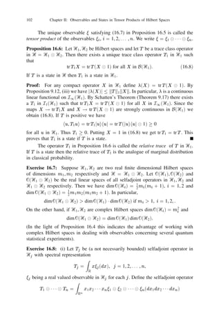
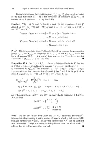
![18 Examples of discrete time quantum stochastic flows 111
Exercise 17.4: Let be an irreducible unitary representation of Sn and let
( ) = tr ( ) be its character. Suppose (1) = d denotes the dimension of the
representation . Define
E =
d X( )U
n! 2S
n
where U is the unitary operator satisfying (17.1). Then E is a projection for
each , E U = U E for all 2 Sn , E1 E2 = 0 if 1 6= 2 and E = 1.
P
(Hint: Use Schur orthogonality relations).
Example 17.5: [74] (i) The volume of the region
1 = f(x1 , x2 , . . . , xN 01 )jxj 0 for all j , 0 x1 + 1 1 1 + xN 01 1g
in ޒ N 01 is [(N 0 1)!]01 .
(ii) Let r1 , . . . , rN be non-negative integers such that r1 + 1 1 1 + rN = n.
Then
Z n! r rN
N + n 0 1 01
p11 1 1 1 pN (N 0 1)!dp1 dp2 1 1 1 dpN 01 =
1 r1 ! 1 1 1 rN ! n
where pN = (1 0 p1 0 p2 0 1 1 1 0 pN 01 ).
This identity has the following interpretation. Suppose all the probability
distributions (p1 , p2 , . . . , pN ) for the occupancy of the cells (1, 2, . . . , N ) by a
particle are equally likely and for any chosen prior distribution (p1 , p2 , . . . , pN ) the
particle obeys Maxwell-Boltzmann statistics. Then one obtains the Bose-Einstein
distribution (17.4) with pj = N , j = 1, 2, . . . , N .
1
Notes
Regarding the role of symmetric and antisymmetric tensor products of Hilbert
spaces in the statistics of indistinguishable particles, see Dirac [29]. For an inter-
esting historical account of indistinguishable particles and Bose-Einstein statistics,
see Bach [11]. Example 17.5 linking Bose-Einstein and Maxwell-Boltzmann statis-
tics in the context of Bayesian inference is from Kunte [74].
18 Examples of discrete time quantum stochastic flows
Using the notion of a countable tensor product of a sequence of Hilbert spaces
with respect to a stabilising sequence of unit vectors and properties of conditional
expectation (see Exercise 16.10, 16.11) we shall now outline an elementary pro-
cedure of constructing a “quantum stochastic flow” in discrete time which is an
analogue of a classical Markov chain induced by a transition probability matrix.
For a Hilbert space Ᏼ any subalgebra Ꮾ Ꮾ(Ᏼ) which is closed under the
involution * and weak topology is called a W 3 algebra or a von Neumann algebra.
If Ᏼi , i = 1, 2 are Hilbert spaces, Ꮾi Ꮾ(Ᏼi ), i = 1, 2 are von Neumann algebras
denote by Ꮾ1
Ꮾ2 the smallest von Neumann algebra containing fX1
X2 jXi 2](https://image.slidesharecdn.com/anintroductiontoquantumstochasticcalculus-130327234248-phpapp01/85/An-introduction-to-quantum-stochastic-calculus-35-320.jpg)
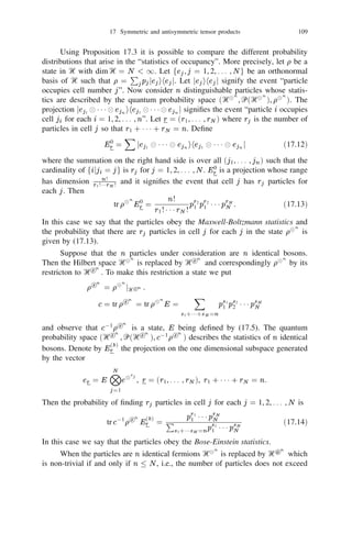
![112 Chapter II: Observables and States in Tensor Products of Hilbert Spaces
Ꮾi , i = 1, 2g in Ꮾ(Ᏼ1
Ᏼ2 ). If is a trace class operator in Ᏼ2 , following
Exercise 16.10, define the operator ( ޅZ ), Z 2 Ꮾ(Ᏼ1
Ᏼ2 ) by the relation
hu, ( ޅZ )v i = tr Z jv ihuj
, u, v 2 Ᏼ1 (18.1)
in Ᏼ1 .
Proposition 18.1: ( ޅZ ) 2 Ꮾ1 if Z 2 Ꮾ1
Ꮾ2 .
Proof: If Z = X1
X2 then (18.1) implies that ( ޅZ ) = (tr X2 )X1 . Thus the
proposition holds for any finite linear combination of product operators in Ꮾ1
Ꮾ2 .
Suppose that = 6pj jej ihej j is a state where pj 0, 6pj = 1 and fej g is an
orthonormal set and w.limn!1 Zn = Z in Ꮾ(Ᏼ1
Ᏼ2 ). Then by (18.1)
lim hu, ( ޅZn )v i = lim
X
n!1 !1 p hu
e , Z v
e i
n
j
j j n j
= 6p hu
e , Zv
e i
j j j
= hu, ( ޅZ )vi for all u, v 2 Ᏼ1 .
In other words ޅis weakly continuous if is a state. Since ޅis linear in
the same property follows for any trace class operator. Now the required result is
immediate from the definition of Ꮾ1
Ꮾ2 .
Let Ᏼ0 , Ᏼ be Hilbert spaces where dim Ᏼ = d 1. Let fe0 , e1 , . . . , ed01 g
be a fixed orthonormal basis in Ᏼ and let Ꮾ0 Ꮾ(Ᏼ0 ) be a von Neumann algebra
with identity. Putting Ᏼn = Ᏼ, n = e0 for all n 1 in Exercise 16.11 construct
the Hilbert spaces Ᏼn] , Ᏼ[n+1 for each n 0. Define the von Neumann algebras
Ꮾn] = fX
1 1 jX 2 Ꮾ0
Ꮾ(Ᏼ
n )g,
[n+ n 0,
Ꮾ = Ꮾ0
Ꮾ(Ᏼ 1 ). [
Property (v) in Exercise 16.11 implies that Ꮾ is the smallest von Neumann algebra
containing all the Ꮾn , n 0. fᏮn] g is increasing in n. By Proposition 18.1 the
[n+1 -conditional expectation ޅn] of Exercise 16.11 maps Ꮾ onto Ꮾn] .
Any algebra with identity and an involution * is called a *-unital algebra.
If Ꮾ1 , Ꮾ2 are *-unital algebras and : Ꮾ1 ! Ꮾ2 is a mapping preserving * and
identity then is called a *-unital map.
Proposition 18.2: Let : Ꮾ0 ! Ꮾ0
Ꮾ(Ᏼ) be a *-unital homomorphism. Define
the linear maps j : Ꮾ0 ! Ꮾ0 by
i
i
j X ( ) = ޅj ih j ((X )),
ej ei 0 i, j d 0 1, X 2 Ꮾ0 (18.2)
Then the following holds:
(1) = , (X 3 ) = (X )3 ; j
P 010 (X ) (Y ) for all X , Y
i i i
(i) j j j i
(X Y ) =
d
(ii) i
j k=
i
k
k
j 2 Ꮾ0 .](https://image.slidesharecdn.com/anintroductiontoquantumstochasticcalculus-130327234248-phpapp01/85/An-introduction-to-quantum-stochastic-calculus-36-320.jpg)
![18 Examples of discrete time quantum stochastic flows 113
Proof: From (18.1) and (18.2) we have
hu, j (X )v i = hu
ei , (X )v
ej i.
i
If X = 1 the right hand side of this equation is hu, v ij . Furthermore
i
3 3
hu, j (X )v i = hu
ei , (X )v
ej i = hv
ej , (X )u
ei i
i
3
= hv , i (X )ui = hu, i (X ) v i.
j j
This proves (i). To prove (ii) choose an orthonormal basis fun g in Ᏼo and observe
that
hu, j (XY )v i = hu
ei , (X ) (Y )v
ej i
i
Xu e Xu e u
3
= h (X )u
ei , (Y )v
ej i
= h
, ( )
k ih
ek , (Y )v
ej i
Xu Xu u Y v
i r r
r ,k
i k
= h , k( ) r ih , j( ) i
X X u Y v
r
k,r
i 3 k
= h k( ) , j( ) i
=h u
X X Y v
k
, i
k( )
k
j( ) i.
k
Proposition 18.3: Let , Ᏼ0 , Ᏼ1 , Ꮾ0 be as in Proposition 18.2. Define the maps
jn : Ꮾ0 ! Ꮾn , n = 0, 1, 2, . . . inductively by
]
jn (X ) =
X
j0 (X ) = X
1 1 , j1 (X ) = (X )
1 2 ,
[
jn01 (k (X ))1n01
i
]
[
jei ihek j
1[n+1 .
(18.3)
0
0 i,j d 1
Then jn is a *-unital homomorphism for every n. Furthermore
ޅn01] jn (X ) = jn01 (0 (X )) for all n 1, X
0
2 Ꮾ0 ,
where ޅn01] is the [n -conditional expectation map of Exercise 16.11.
Proof: We prove by induction. For n = 0, 1 it is immediate. Let n 2. Then by
Xj 0 0
(i) in Proposition 18.2 and the induction hypothesis we have
jn (1) = i
1 ( j )1n 1]
j i ih j j
e e 1[n+1
Xe e
n
i,j
= 0
1n 1]
j i ih i j
1[n+1 = 1
i](https://image.slidesharecdn.com/anintroductiontoquantumstochasticcalculus-130327234248-phpapp01/85/An-introduction-to-quantum-stochastic-calculus-37-320.jpg)
![114 Chapter II: Observables and States in Tensor Products of Hilbert Spaces
and
jn (X )3 =
X jn01 (i (X 3 ))1n01]
j
je ihe j
1
j i [n+1
i,j
= jn (X ).
3
X 0
By (ii) in Proposition 18.2 and induction hypothesis we have
jn (X )jn (Y ) = jn 1 (j (X ))jn01 (` (Y ))1n01]
i k
je ihe j
1
k
X 0X
j i ` [n+1
i,j ,k,`
= jn 1 k (X )` (Y ))1n01]
i k
je ihe j
1
X0
i ` [n+1
i,` k
= jn 1 (` (XY ))1n01]
i
je ihe j
1
i ` [n+1 .
i,`
This proves the first part. By the definition of ޅn] in Exercise 16.11 and the fact
that he0 , jei ihej je0 i = 0 j , the second part follows from (18.3).
i 0
Corollary 18.4: Let fjn , n 0g be the *-unital homomorphisms of Proposition
18.3. Write T = 0 . Then for 0 n0 n1 1 1 1 nk 1, Xi 2 Ꮾ0 , 1 i k
0
ޅn0 ] jn1 (X1 )jn2 (X2 ) 1 1 1 jnk (Xk ) =
jn0 (T n1 0n0 (X1 T n2 0n1 (X2 1 1 1 (X 01 T k 0 (18.4)
k
n 0
nk 1
(X )) 1 1 1)
Proof: By Exercise 16.11 ޅn0 ] = ޅn0 ] ޅnk01 ] . Since jn1 (X1 ) 1 1 1 jnk01 (Xk01 ) is
an element of Ꮾnk01] it follows from the same exercise that
ޅn0 ] jn1 (X1 ) 1 1 1 jnk (Xk )
(18.5)
= ޅn0] jn1 (X1 ) 1 1 1 jnk01 (Xk01 )ޅnk01 ] (jnk (Xk )).
Since ޅnk01 ] = ޅnk01] ޅnk01 +1] 1 1 1 ޅnk 01] it follows from Proposition 18.3 that
ޅnk01 ] jnk (Xk ) = jnk01 (T nk 0nk01 (X )).
Substituting this in (18.5), using the fact that jnk01 is a homomorphism and re-
peating this argument successively we arrive at (18.4).
Proposition 18.5: The map T = 0 from Ꮾ0 into itself satisfies the following:
0
P
(i) T is a *-unital linear map on Ꮾ(Ᏼ0 ); (ii) for any Xi , Yi 2 Ꮾ0 , 1 i k,
3 3
1i,j k Yi T (Xi Xj )Yj 0 for every k . In particular, T (X ) 0 whenever
X 0.](https://image.slidesharecdn.com/anintroductiontoquantumstochasticcalculus-130327234248-phpapp01/85/An-introduction-to-quantum-stochastic-calculus-38-320.jpg)
![18 Examples of discrete time quantum stochastic flows 115
Proof: Since is a *-unital homomorphism from Ꮾ0 into Ꮾ0
Ꮾ(Ᏼ) and
T (X ) = ޅje0 ihe0 j ((X )), (i) is immediate from Exercise 16.10. Using the same
X
exercise once again we have
Yi3 T (Xi Xj ))Yj =
3
X Yi3 ޅje0 ihe0 j ((Xi )3 (Xj ))Yj
i,j
=
i,j
ޅje0 ihe0 j (f
X (Xi )Yi
1g f 3
X (Xj )Yj
1g) 0.
i j
Putting k = 1, Y1 = 1, X1 = X in this relation we get the last part.
We may now compare the situation in Proposition 18.3, Corollary 18.4 and
Proposition 18.5 with the one that is obtained in the theory of classical Markov
chains. Consider a Markov chain with state space S = f1, 2, . . . , N g and transition
probability matrix P = ((pij )), 1 i, j N . Denote by B1 the *-unital
commutative algebra of all bounded complex valued measurable functions on the
space S 1 = S0 2 S1 21 1 12 Sn 21 1 1 where Sn = S for every n. Let Bn] B1 be
the *-subalgebra of all functions which depend only on the first n + 1 coordinates.
Denote by ޅn] the conditional expectation map determined by
(ޅn] g )(i0 , i1 , . . . , in ) = (ޅg jX0 = i0 , X1 = i1 , . . . , Xn = in )
where X0 , X1 , . . . is the Markov chain starting in the state X0 = i0 with stationary
transition probability matrix P . For any function f on S define
jn (f )(i) = f (in ) where i = (i0 , i1 , . . . , in , . . .) 2S 1
.
Then jn is a *-unital homomorphism from B0 into Bn] and the Markov property
implies that
ޅn0] jn1 (f1 )jn2 (f2 ) 1 1 1 jnk (fk ) =
(18.6)
jn0 (T n1 0n0 (f1 (T n2 0n1 f2 ( 1 1 1 (fk 01 T nk 0nk01 (fk )) 1 1 1)
where
(T f )(i) =
XN
pij f (j ), f 2 B0 = B0 , ]
j =1
n0 n1 111 2
nk and f1 , . . . , fk B0 . T is a *-unital positive linear map on
B0 . Then (18.4) is the non-commutative or quantum probabilistic analogue of the
classical Markov property (18.6) expressed in the language of *-unital commuta-
f
tive algebras. For this reason we call the family jn , n 0 of homomorphisms in g
Proposition 18.3 a quantum stochastic flow induced by the *-unital homomorphism
: Ꮾ0 !
Ꮾ0 Ꮾ(Ᏼ).
Proposition 18.6: Suppose that the von Neumann algebra Ꮾ0 in Proposition 18.3
is abelian. Then for any X , Y 2 Ꮾ0 , m, n 0
[jm (X ), jn (Y )] = 0. (18.7)](https://image.slidesharecdn.com/anintroductiontoquantumstochasticcalculus-130327234248-phpapp01/85/An-introduction-to-quantum-stochastic-calculus-39-320.jpg)
![116 Chapter II: Observables and States in Tensor Products of Hilbert Spaces
Proof: Since jn is a homomorphism we have [jn (X ), jn (Y )] = jn ([X , Y ]) = 0.
Thus (18.7) is trivial if m = n. Suppose m n. By induction on (18.3) we have
jn (X )
X =
j
i
m k
([
1
1
111
in0m
k
n0m (X ))1 m
] i k
je 1 ihe 1 j
1 1 1
je in0m ekn0m
ih j
1[n+1
0 i1 ,i2 ,... ,
0
k1 ,k2 ,... , d 1
from which it follows that
X m m ki
n
[j (X )
j
,j
([
(Y )] =
1
1
111
i
n0m (X ), Y ])1
kn0m m ] i k
je 1 ihe 1 j
1 1 1
je in0m ekn0m
ih j
1[n+1
i1 ,i2 ,...
k1 ,k2 ,...
= 0 for all X , Y 2 Ꮾ0 .
If Ꮾ0 is abelian and X1 , X2 , . . . , Xk is any finite set of selfadjoint elements
in Ꮾ0 then jn1 (X1 ), jn2 (X2 ), . . . , jnk (Xk ) is a commuting family of observables
and hence possesses a joint distribution in ޒk in any state on the countable
tensor product Ᏼ0
fᏴ
Ᏼ
1 1 1g where the Hilbert space within the braces
f g is with respect to the constant stabilising sequence of unit vectors e0 . For
any state 0 in Ᏼ0 , the family fjn (X )jX 2 Ꮾ0 , n 0g can be interpreted as a
classical Markov flow in the state 0
je0
e0
1 1 1ihe0
e0
1 1 1 j.
Example 18.7: Let (S , Ᏺ, ) be any measure space and let j : S ! S be
measurable maps satisfying 01 , 0 j d 0 1. Suppose pj : S !
j P
[0, 1], 0 j d 0 1 are measurable functions satisfying
j pj (x) 1. Let
1 () Ꮾ(L2 ()) when bounded measurable functions are considered
Ꮾ0 = L
as bounded multiplication operators. We write Ᏼ0 = L2 (), Ᏼ = ރd and choose
fe0 , e1 , . . . , ed01 g to be the canonical orthonormal basis in Ᏼ. Define the map
T : Ꮾ0 ! Ꮾ0 by
X p f o
d0 1
Tf = j j 18.8)
(
j =0
where o denotes composition. The map T can be interpreted as the transition op-
erator of a Markov chain with state space S for which the state changes in one
step from x to one of the states 0 (x), 1 (x), . . . , d01 (x) with respective proba-
bilities p0 (x), p1 (x), . . . , pd01 (x). However, it is possible that i (x) = j (x) for
some i 6= j . If S is a finite set of cardinality k it can be shown that every Markov
transition operator is of the form (18.8) with being counting measure. In many
practically interesting models of classical probability d is small.
Consider a unitary d 2 d matrix valued measurable function U on S for
which U = ((uij )), 0 i, j d 0 1, u0j = pj for all j . For example one may
p](https://image.slidesharecdn.com/anintroductiontoquantumstochasticcalculus-130327234248-phpapp01/85/An-introduction-to-quantum-stochastic-calculus-40-320.jpg)
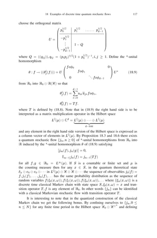
![18 Examples of discrete time quantum stochastic flows 117
choose the orthogonal matrix
0 p1=2 p1=2
1 1
1
. . . . . . pd=21
0
B 0 1=2
B C
C
U = B 0p.1
B
B
C
C
C
@ .. 10Q A
0p 0 1=2
d 1
where Q = ((qij )), qij = (pi pj )1=2 (1 + p0=2 )01 , i, j
1
1. Define the *-unital
homomorphism
0 fo0 0
1
: f ! ((j (f ))) = U @
i fo1 A U3 (18.9)
..
0 . fod01
from Ꮾ0 into Ꮾ0
Ꮾ(Ᏼ) so that
X
d01
(f ) =
i
j uir ujr for ,
r=0
0 (f ) = T f .
0
where T is defined by (18.8). Note that in (18.9) the right hand side is to be
interpreted as a matrix multiplication operator in the Hilbert space
L2 ()
ރd = | 2 () 8 1{z1 8 L2 (}
L 1 )
d0fold
and any element in the right hand side version of the Hilbert space is expressed as
a column vector of elements in L2 (). By Proposition 18.3 and 18.6 there exists
a quantum stochastic flow fjn , n 0g of *-unital homomorphisms from Ꮾ0 into
Ꮾ induced by the *-unital homomorphism of (18.9) satisfying
[jm (f ), jn (g)] = 0,
] ޅn01 jn (f ) = jn01 (T f )
for all f , g 2 Ꮾ0 = L1 (). If S is a countable or finite set and is
the counting measure then for any x 2 S , in the quantum theoretical state
x
e0
e0
1 1 1 in L2 ()
Ᏼ
Ᏼ
1 1 1 the sequence of observables j0 (f ) =
f , j1 (f ), . . . , jn (f ), . . . has the same probability distribution as the sequence of
random variables f (0 (x, ! )), f (1 (x, ! )), f (n (x, ! )), . . . where fn (x, ! )g is a
discrete time classical Markov chain with state space S , 0 (x, ! ) = x and tran-
sition operator T , f is any element of Ꮾ0 . In other words fjn g can be identified
with a classical Markovian stochastic flow with transition operator T .
It is interesting to note that in the quantized construction of the classical
Markov chain we get the following bonus. By confining ourselves to fjn , 0
n N g for any finite time period in the Hilbert space Ᏼ0
Ᏼ
n and defining](https://image.slidesharecdn.com/anintroductiontoquantumstochasticcalculus-130327234248-phpapp01/85/An-introduction-to-quantum-stochastic-calculus-41-320.jpg)
![118 Chapter II: Observables and States in Tensor Products of Hilbert Spaces
the conditional expectations ޅn] with respect to an arbitrary unit vector , in Ᏼ
replacing e0 , we get a Markov flow with the property
ޅn0 ] jn1 (f1 ) 1 1 1 jnk (fk ) = jn0 (T n1 0n0 (f1 T n2 0n1 (f2 1 1 1 (fk01 T
nk 0nk01 (f
k )) 1 1 1)
for all 0 n0 n1 1 1 1 nk N T
XeU
where is the Markov transition operator
0
d 1
T f= jh j, (1) ij
2
foj .
j =0
T describes the chain where the state changes from x to one of the states
0 (x), 1 (x), . . . , d01 (x) with respective probabilities jhej , U (x) ij2 , j = 0, 1,
. . . , d 0 1. Thus a quantum probabilistic description enables us to describe a whole
class of Markov chains with transition operators T , 2 Ᏼ, k k = 1 within the
N
framework of a single Hilbert space Ᏼ0
Ᏼ
if we confine ourselves to the
finite time period [0, N ].
Example 18.8: We examine Example 18.7 when d = 2. Denote the maps 0 and
1 on S by and respectively. Write p0 = p, p1 = q so that p + q = 1. Then
the *-unital homomorphism in (18.9) assumes the simple form
i
(f ) = ((j (f ))) = pfo + qfo p
pq (fo 0 fo) (18.10)
p
pq (fo 0 fo) qfo + pfo
when
U= pp p
q .
0
p
q p
p
Define
an = 1n01 ]
j e0 ihe1 j
1 n [ +1 ,
ay = 1n01
n ]
j e1 ihe0 j
1 n [ +1 , n = 1, 2, . . . ,
so that
an ay = 1n01
n ]
j e0 ihe0 j
1 n [ +1 ,
ay an = 1n01
n ]
j e1 ihe1 j
1 n [ +1 ,
and an ay + an an = 1 for all
n
y n 1. Then the flow fjn , n 0g induced by in
(18.3) assumes the form
jn (f ) = jn01 (T f ) + jn01 (Lf )(an + ay ) + jn01 (Kf )ay an
n n (18.11)
for all f 2 L 1 (), n 1 where
T f = pfo + qfo ,
(18.12)
Lf = pq (fo 0 fo), Kf = (p 0 q )ffo 0 fog
p](https://image.slidesharecdn.com/anintroductiontoquantumstochasticcalculus-130327234248-phpapp01/85/An-introduction-to-quantum-stochastic-calculus-42-320.jpg)
![18 Examples of discrete time quantum stochastic flows 119
If An = 0 for n = 0 and a1 + + an for n 1 and 3n = 0 for n = 0 and
111
ay a1 + + ay an for n 1 we may express (18.11) in the form
1 111 n
jn (f ) = jn01 (Tf )+jn01 (Lf )(An An01 +Ay Ay 01 )+jn01 (Kf )(3n 3n01 )
0 n n 0 0
(18.13)
where An , Ay and 3n , n 0 are three martingales with respect to the conditional
n
expectations ޅn] (see Exercise 16.12). In Chapter III we shall treat continuous
time analogues of flows satisfying (18.13) where difference equations will become
differential equations.
Example 18.9: (Hypergeometric model) Consider an urn with a white balls and
b black balls. Draw a ball at random successively without replacement. The state
of the Markov chain at any time is denoted (x, y ) where x is the number of white
balls and y is the number of black balls. Then
S = (x, y) 0 x a, 0 y b
f j g
is the state space. Define maps , on S by
8 (x 1, y) if x 0
0
(x, y) = : (0, y 1) if x = 0, y 0,
0
(0, 0) if x = 0, y = 0,
8 (x, y 1) if y 0,
0
(x, y) = : (x 1, 0) if y = 0, x 0,
0
(0, 0) if x = y = 0.
Define x if x 0,
p(x, y) = x+y
1
if x = 0.
2
Then
8 x y
x + y f (x 1, y) + x + y f (x, y 1)
x 0, y 0,
0 0 if
(Tf )(x, y) = f (x 1, 0)
0 if x 0, y = 0,
f (0, y 1)
: 0 if x = 0, y 0,
f (0, 0) if x = 0, y = 0.
We may call f jn , n 0 defined by the *-unital homomorphism in (18.10)–
g
(18.12) the hypergeometric flow.
Example 18.10: (Ehrenfest’s model) There are two urns with a and b balls so
that a + b = c. One of the c balls is chosen at random and shifted from its urn to
the other. The state of the system is the number of balls in the first urn. Then
S= f 0, 1, 2, . . . , cg.
Define the maps , on S by
(x) = x 1 0 if x 0,
if x = 0,
nx + 1
1
if x c,
(x) = c 1 0 if x = c.](https://image.slidesharecdn.com/anintroductiontoquantumstochasticcalculus-130327234248-phpapp01/85/An-introduction-to-quantum-stochastic-calculus-43-320.jpg)
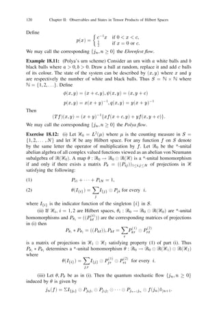
![18 Examples of discrete time quantum stochastic flows 121
If
is the unit vector in Ᏼ with respect to which the conditional expectation maps
ޅn] , n 0 are defined then
ޅn01] jn (f ) = jn01 (T f ) where (T f )(i) =
Xp f (j) p
ij , ij = h
, Pij
i.
j
Example 18.13: [115] Let G be a compact second countable group and let
g ! Lg denote its left regular representation in the complex Hilbert space L2 (G)
of all absolutely square integrable functions on G with respect to its normalised
Haar measure so that (Lg f )(x) = f (g 01 x), f 2 L2 (G). Denote by Ꮾ0 the von
Neumann algebra generated by fLg jg 2 Gg and its centre by Z0 . Let 0(G) denote
the countable set of all characters of irreducible unitary representations of G. For
any 2 0(G) let U be an irreducible unitary representation of G with character
and dimension d(). If 1 , 2 2 0(G) the map g ! Ug 1
Ug 2 , g 2 G
defines a unitary representation which decomposes into a direct sum of irreducible
representations. Denote by m(1 , 2 ; ) the multiplicity with which the type U
appears in such a decomposition of U 1
U 2 . Define
m(, 2 ; 1 )d(2 )
p1 ,2 =
.
d()d(1 )
Then Xp
1 ,2 = 1 for each , 1 2 0(G).
2 20(G)
In other words, for every fixed 2 0(G), the matrix P = ((p1 ,2 )) is a
stochastic matrix over the state space 0(G). In each row of P all but a finite
M
number of entries are 0 and each entry is rational. Thanks to the Peter-Weyl
Theorem L2 (G) admits the Plancherel decomposition
L2 (G) = Ᏼ
20(G)
where dim Ᏼ = d()2 , Lg leaves each Ᏼ invariant and Lg jᏴ , g 2 G is a
direct sum of d() copies of the representation U . If denotes the orthogonal
projection onto the component Ᏼ then
= d()
Z (g)L dg g .
G
Fix 0 2 0(G). Let U 0
act in the Hilbert space Ᏼ. Denote by
N
the state
d(0 )01 I in Ᏼ. Fix a positive integer N and consider in Ᏼ
the increasing
sequence of von Neumann subalgebras
= fX
1 n 1,N jX 2 Ꮾ(Ᏼ
n )g, n = 1, 2, . . . , N
Ꮾn] [ + ]
N b0a+
where ᏮN = Ꮾ(Ᏼ
) and 1 a,b denotes the identity in Ᏼ
1
] [ ] , the tensor
N
product of the a-th, a + 1-th,. . . , b-th copies of Ᏼ in Ᏼ
. Consider the conditional
expectation maps ޅn] : ᏮN ] ! Ꮾn ] defined by
ޅn] X = (
ޅN 0n X )
1 n [ +1,N ] , 1nN 01](https://image.slidesharecdn.com/anintroductiontoquantumstochasticcalculus-130327234248-phpapp01/85/An-introduction-to-quantum-stochastic-calculus-45-320.jpg)
![122 Chapter II: Observables and States in Tensor Products of Hilbert Spaces
(see Exercise 16.10) so that
ޅn] X1
1 1 1
XN = (5N n
i = +1
tr Xi)(X1
1 1 1
Xn)
1 n [ +1, N ]
X
for all i 2 Ꮾ(Ᏼ). By the Peter-Weyl Theorem there exists a unique *-unital
j
homomorphism n 0 : Ꮾ0 ! Ꮾn] satisfying
(i) jn (Lg ) = (Ug )
n
1 n 1,N
0 0
[ + ]
ޅn01 jn (X ) = jn01 (T (X )) for all X 2 Ꮾ0 where
X p
0
(ii) ]
T (Lg ) = d(0)01 0(g)Lg , T ( ) = 0
0, 0 .
2 G0 0( )
Z G
j Z j X
(iii) The centre 0 of Ꮾ0 is generated by f j 2 0( )g and [ m0 ( ), r 0 ( )] =
0 for all Z Z X m n
2 0 , 2 Ꮾ0 , . In particular, the family f n 0 ( )j1
j Z
n Nz Z j n N
, 2 0 g is commutative and hence f n 0 jZ0 , 1 g induces
G
a classical Markov chain with state space 0( ) and transition probability
P
matrix 0 for every 0 2 0( ). G
(iv) When G = SU (2) and n denotes the character of the unique equivalence
class of an irreducible unitary representation of dimension n the Clebsch-
Gordan formula implies that
8i01
2 j = i 0 1,
= i +i 1
if
pi2 ,j
: 2i if j = i + 1,
0 otherwise.
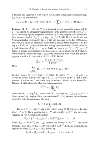
Exercise 18.14: Let (S , Ᏺ, ) be as in Example 18.7. Suppose that
X
d0 1 X
d0 1
T1f = pifoi, T2f = qi fo i
i=0 i
=0
are two Markov transition operators as described in (18.8) and
0 fo 0
1
B fo C U0 ,
0
(f ) = U B
1 @ ..
.
1
C
A 1
0 fod01
0 fo 0
1
B fo CV 0 ,
0
(f ) = V B
2 @ ..
.
1
C
A 1
0 fo d01](https://image.slidesharecdn.com/anintroductiontoquantumstochasticcalculus-130327234248-phpapp01/85/An-introduction-to-quantum-stochastic-calculus-46-320.jpg)
![19 The Fock Spaces 123
are the *-unital homomorphisms corresponding to (18.9). Define
V
W = 0U cos V 3U 3sincos ,
V 3 sin V
0 fo 0 0
1
B
B
..
. C
C
B fod0 C
(f ) = W B
B
B
1
fo
C W 01
C
C
B
@
0
.. C
A
.
0 fo d01
where is any fixed angle. Then W
is a unitary matrix valued function and is
T T
a *-unital homomorphism for which 0 = 1 cos2 + 2 sin2 . Thus the Markov
0
transition operator of the quantum stochastic flow induced by is a superposition
(or convex combination) of the two transition operators i , = 1, 2. T i
Notes
The idea of describing a general quantum stochastic process in terms of a time
j j
indexed family f n g or f t g of *-unital homomorphisms from a *-unital initial or
~
system algebra Ꮾ0 into a larger *-unital algebra Ꮾ made up of Ꮾ0 and noise or heat
bath elements has its origin in Accardi, Frigerio and Lewis [6] modelled on the
description of classical processes by Nelson (J. Funct. Anal., 12 (1973) 97–112,
211–277) and Guerra, Rosen and Simon (Ann. Math., 101 (1975) 111–259).
For a detailed account of Markov chains (or discrete time flows) in *-algebras
of the form Ꮾ0
Ꮾ
Ꮾ
1 1 1 where Ꮾ0 is the initial or system algebra and Ꮾ is the
noise algebra see Kummerer [71,73]. The account given here is in anticipation of
Evans-Hudson flows which are discussed in Section 28. It is based on Parthasarathy
[112] and inspired by Meyer [91]. Example 18.9–18.11 are based on classical
probability theory as described in Feller [40]. Example 18.12 was suggested to
me by B.V.R. Bhat. Example 18.13 is based on the work of Biane [22], von
Waldenfels [138] and Parthasarathy [115].
19 The Fock Spaces
In Section 16–18 we saw how the notion of tensor products of Hilbert spaces
enables us to combine several quantum probability spaces into one. In this context
there is yet another basic construction leading to the combination of an “indefinite”
number of such systems. This idea is illustrated by first raising the following
question: if the events concerning the dynamics of a single particle are described
by the elements of ᏼ(Ᏼ) where Ᏼ is a separable Hilbert space, how does one
construct the Hilbert space for an indefinite number of such particles in a system
where the indefiniteness is due to the fact that “births” and “deaths” of particles
take place or, equivalently, particles are being “created” and “annihilated” subject](https://image.slidesharecdn.com/anintroductiontoquantumstochasticcalculus-130327234248-phpapp01/85/An-introduction-to-quantum-stochastic-calculus-47-320.jpg)

![128 Chapter II: Observables and States in Tensor Products of Hilbert Spaces
Proposition 19.7: Let Ᏼ1 , Ᏼ2 be Hilbert spaces and let Ᏼ = Ᏼ1 8 Ᏼ2 . Then
there exists a unique unitary isomorphism U : 0a (Ᏼ1 8 Ᏼ2 ) ! 0a (Ᏼ1 )
0a (Ᏼ2 )
satisfying the relations:
U [(m + n)!]1=2 u1 ^ 1 1 1 ^ um ^ v1 ^ 1 1 1 ^ vn
(19.5)
= f(m!)1=2 u1 ^ 1 1 1 ^ um g
f(n!)1=2 v1 ^ 1 1 1 ^ vn g
for all ui 2 Ᏼ1 , vj 2 Ᏼ2 , 1 i m, 1 j n, m = 1, 2, . . . , n = 1, 2, . . . and
U 8 = 81
82 , 8, 81 , 82 being the vacuum vectors in 0a (Ᏼ), 0a (Ᏼ1 ), 0a (Ᏼ2 )
respectively.
Proof: Once again, as in the proof of Proposition 19.6, we assume without loss
of generality that Ᏼ1 , Ᏼ2 are orthogonal subspaces of Ᏼ. Let
S = f8, [(m + n)!]1=2 u1 ^ 1 1 1 ^ um ^ v1 ^ 1 1 1 ^ vn jui 2 Ᏼ1 , vj 2 Ᏼ2 , g
1 i m, 1 j n, m = 1, 2, . . . ; n = 1, 2, . . .g,
S1 = f81 , (m!)1=2 u1 ^ 1 1 1 ^ um , ui 2 Ᏼ1 , 1 i m, m = 1, 2, . . .g,
S2 = f82 , (n!)1=2 v1 ^ 1 1 1 ^ vn , vi 2 Ᏼ1 , 1 i n, n = 1, 2, . . .g.
By Proposition 19.3, S , S1 , S2 are total in 0a (Ᏼ), 0a (Ᏼ1 ), 0a (Ᏼ2 ) respectively.
Furthermore, the set fu
v ju 2 S1 , v 2 S2 g is total in 0a (Ᏼ1 )
0a (Ᏼ2 ). Thus
it suffices to show that the map U defined by (19.5) is scalar product preserving.
Let ui , uk 2 Ᏼ1 , 1 i m, 1 k m , vj , v` 2 Ᏼ2 , 1 j n, 1 ` n .
0 0 0 0
We now consider three different cases:
Case 1: m + n 6= m0 + n0 .
Define u1 ^1 1 1^ um = 81 , v1 ^1 1 1^ vn = 82 , u1 ^1 1 1^ um ^ v1 ^1 1 1^ vn = 8
when m = n = 0. Then we see that since u1 ^ 1 1 1 ^ um ^ v1 ^ 1 1 1 ^ vn and
u01 ^ 1 1 1 ^ u0m0 ^ v1 ^ 1 1 1 ^ v1 ^ 1 1 1 ^ vn0 are m + n and m0 + n0 -particle vectors,
0 0 0
they are orthogonal. Furthermore, either m 6= m0 or n 6= n0 and hence
hu1 ^ 1 1 1 ^ um , u1 ^ 1 1 1 ^ um ihv1 ^ 1 1 1 ^ vn , v1 ^ 1 1 1 ^ vn i = 0.
0 0
0
0 0
0 (19.6)
Case 2: m + n = m0 + n0 , m 6= m0 .
Without loss of generality let m m , n n . Then (19.6) holds. On the
0 0
other hand, writing
(u1 , . . . , um , v1 , . . . , vn ) = (w1 , . . . , wm+n ),
(u1 , . . . , um , v1 , . . . , vn ) = (w1 , . . . , wm+n )
0 0
0
0 0
0
0 0
we observe that the matrix ((hwi , wj i)), 1 i, j m + n has the partitioned
0
form 0A Bm2(m 0m)
1
@ m02m
0
C m 0m 2 n A
0
0 ( 0 ) 0
0 0 Dn 2n 0 0](https://image.slidesharecdn.com/anintroductiontoquantumstochasticcalculus-130327234248-phpapp01/85/An-introduction-to-quantum-stochastic-calculus-52-320.jpg)
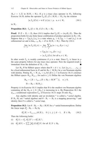
 = ezx0 z 1
2
2
for all z 2 .ރ (19.8)](https://image.slidesharecdn.com/anintroductiontoquantumstochasticcalculus-130327234248-phpapp01/85/An-introduction-to-quantum-stochastic-calculus-53-320.jpg)
 = exp(z 1 x 0
1 X k
zj )
2
(19.9)
P
2
j =1
Then U is a unitary isomorphism between L2 (
k
where z 1 x = j zj xj . )
is the countably infinite cardinal and correspondingly
k
and 0s (ރk ).When k
is the countable cartesian product of standard normal distributions we obtain a
unitary correspondence between the L2 -space of an independent and identically
distributed sequence of standard Gaussian random variables and the boson Fock
space 0s (`2 ), `2 denoting the Hilbert space of absolutely square summable se-
quences. This leads us to the connection between Brownian motion and the boson
Fock space.
Example 19.9: Let fw(t)jt 0g be the standard Brownian motion stochastic
process described by the Wiener probability measure P on the space of continuous
functions in [0, 1). Then w (0) = 0 and for any 0 t1 t2 1 1 1 tk
1, w(t1 ), w(t2 ) 0 w(t1 ), . . . , w(tk ) 0 w(tk01 ) are independent Gaussian random
R
variables with mean 0 and (ޅw(t) 0 w(s))2 = t 0 s. For any complex valued
function f in L2 ( ) +ޒwhere )1 ,0[ = +ޒis equipped with Lebesgue measure, let
1 fdw denote the stochastic integral (in the sense of Wiener) of f with respect to
0
the path w of the Brownian motion. Then the argument outlined in Example 19.1
Z Z
shows that there exists a unique unitary isomorphism U : 0s (L2 ( ! )) +ޒL2 (P )
satisfying
1 1 1
[U e(f )](w ) = exp( fdw 0 f (t)2 dt). (19.10)
0 2 0
For any t 0, let ft] = f I[0,t] which agrees with f in the interval [0, t] and
vanishes in the interval (t, 1). Then
[U e(ft] )](w ) = exp(
Z t
f dw 0
1
Z t
f (s)2 ds), t0 (19.11)
0 2 0](https://image.slidesharecdn.com/anintroductiontoquantumstochasticcalculus-130327234248-phpapp01/85/An-introduction-to-quantum-stochastic-calculus-54-320.jpg)
![19 The Fock Spaces 131
where the right hand side as a stochastic process is the well-known exponential
martingale of classical stochastic calculus.
A multidimensional analogue of this example can be constructed as follows.
Suppose fw(t) = (w1 (t), w2 (t), . . . , wn (t))jt 0g is the n-dimensional standard
Brownian motion process whose probability measure in the space of continuous
sample paths with values in ޒn is P
. Let fej j1 j ng be the canonical
n
n
basis of column vectors in . ރThen there exists a unique unitary isomorphism
U : 0s (L2 (ރ
) +ޒn ) ! L2 (P
n ) satisfying
X n
Ue f (] )
[ ( t
j
ej )](w) = exp
X n
f
Z t
f (j) (s)dwj (s) 0 1
Z t
f (j) (s)2 dsg
2
=j 1 j =1 0 0
for all f (j ) in L2 ( ,) +ޒj = 1, 2, . . . , n.
Example 19.10: Let be the Poisson distribution with mean value in the space
Z+ of non-negative integers. In L2 () consider the generating function of the
Charlier-Poisson polynomials defined by
p z 1
z )x = X z n (, x), x 2 Z .
e0 (1 + p
n! n + (19.12)
n=0
Then there exists a unique unitary isomorphism U : 0s ( ! )ރL2 () satisfying
[Ue(z )](x) = e
0p z (1 + p )x for all z 2 .ރ
z (19.13)
Under this isomorphism
U (1, 0, 0, . . .) = 1,
U (0, 0, . . . , 0, 1, 0, . . .) = (n!)0 n (, x), n = 1, 2, . . .
1
2
where 1 appears in the n-th position and n = 0, 1, 2, . . . , and in particular,
f(n!)0 n (, x)jn = 0, 1, 2, . . .g is an orthonormal basis in L2 ().
1
2
Example 19.11: Let fN (t)jt 0g be the Poisson process with stationary inde-
pendent increments, right continuous trajectories and intensity parameter and let
its distribution be described by the probability measure P . Then
P fN (t) 0 N (s) = j g = e0(t0s) [(t j ! s)] , j = 0, 1, 2, . . .
0 j
and the conditional distribution of the jump points 0 1 2 1 1 1 n t,
given the fact that the process has n jumps in [0, t], is uniform in the simplex
fsj0 s1 1 1 1 sn tg. This enables us to construct a natural unitary
isomorphism U between 0s (L2 ( )) +ޒand L2 (P ) by putting for every t 0
R
[Ue(ft] )](N ) = e
0p f (s)ds 5 t
[N (s+) 0 N (s0)]
f (s)g (19.14)
0st f1 + p
0](https://image.slidesharecdn.com/anintroductiontoquantumstochasticcalculus-130327234248-phpapp01/85/An-introduction-to-quantum-stochastic-calculus-55-320.jpg)
![132 Chapter II: Observables and States in Tensor Products of Hilbert Spaces
(where N (00) = 0) for all f in L2( ) +ޒand f t] is defined as in (19.11). Indeed,
hUe(f ), Ue(g )i =
t] t]
p R 1
e0 (t!) 2
X
e0
t n
[f (s)+g (s)]ds t
0
n n=0
Z
n!t0 n fps ) )(1 + gps ) )ds 1 1 1 ds
( ( n
5j =1 (1 +
j j
0 111 n s1 s t 1 n
p Z t Z
f (s) g(s) t
= expf0 [f (s) + g (s)]ds 0 t + (1 + p )(1 + p )dsg
Z
0 0
t
= exp f (s)g(s)ds = he(f ), e(g )i. t] t]
0
L P
In 2 ( ) the totality of the set of random variables occurring on the right hand
f L
side of (19.14) as varies in 2 ( ) +ޒand in +ޒis an exercise for the reader. t
S
Example 19.12: [51] Let ( , Ᏺ, ) be a non-atomic, -finite and separable mea-
S
sure space. For any finite set denote by # its cardinality. Let 0( ) be the S
S
space of all finite subsets of and 0n ( ) = f j , # = g, 00 ( ) = f;g S S n S
S
where ; is the empty subset of . (Thus the empty subset of is a point in 0( )!). S S
For any symmetric measurable function on n define the function n on 0( ) f S f S
by
8
( 1 , . . . , n ) if # = , fs s n
f () = :
n = fs1 , . . . , s g,
n
0 otherwise.
Let Ᏺ0 be the smallest -algebra which makes all such functions n measurable f
n
for = 1, 2, . . . . Define the measure 0 on Ᏺ0 as follows. Let 1n n denote S
s s s s s
the subset f = ( 1 , . . . , n )j i 6= j for 6= g. The non-atomicity of implies i j
that
( n n1n ) = 0. For any 2 Ᏺ0 put
S E
n
1
X1 Z
(E ) = I (;) +
0 E
n! I j E 0 n (S ) ( fs1 , . . . , s g)(ds1 ) 1 1 1 (ds
n n) . (19.15)
n=1 1 n
Then
is a -finite measure whose only atom is ; with mass at ; being unity.
S S
0
(0( ), Ᏺ0 , 0 ) is called the symmetric measure space over ( , Ᏺ, ) in the sense
of A. Guichardet [51]. We write = d d
( ) when integration is with respect to
0
0.
For any function f on S let
() = 1 if = ;,
2 f (s)
f (19.16)
5s otherwise.](https://image.slidesharecdn.com/anintroductiontoquantumstochasticcalculus-130327234248-phpapp01/85/An-introduction-to-quantum-stochastic-calculus-56-320.jpg)
![19 The Fock Spaces 133
Then f g = fg and f = f . If f is integrable with respect to then (19.15)
X Z
implies
Z 1
f ( )d = 1 + n 5n=1 f (sj )(ds1 ) (dsn )
1
Z fd
j 111
0(S ) ! Sn
n=1 (19.17)
= exp .
S
Now consider the Hilbert space L2 (0 ). It is an exercise for the reader to show
Z ()d = Z
that ff jf 2 L2 ()g is total in L2 (). Equation (19.17) implies that
f , g i =
Z fg d
h f g fg ( )d = exp .
S
This at once enables us to see the unitary isomorphism U : 0s (L2 ()) ! L2 (0 )
satisfying the relations
[Ue(f )]() = f () for all f in L2 ().
Exercise 19.13: Let Ᏼ = ރn or `2 according to whether n is the finite or countably
infinite cardinal. Suppose fj jj = 1, 2, . . .g is an n-length sequence of independent
and identically distributed Bernoulli random variables assuming the values 61 with
equal probability. Choose and fix an orthonormal basis fe1 , e2 , . . .g in Ᏼ. Then
there exists a unique unitary isomorphism U : 0a (Ᏼ) ! L2 (P ) satisfying
U 8 = 1,
U (k!)1=2 ej1 ^ ej2 ^ 1 1 1 ^ ejk = j j 1 2
111 jk , j1 j2 1 1 1 jk ,
k 1 + dim Ᏼ where 8 is the vacuum vector and P is the probability measure
of the sequence fj g. (Hint: Use Proposition 19.3.)
Exercise 19.14: Let be any (not necessarily non-atomic!) -finite measure
in .)1 ,0[ = +ޒDefine the measurable space (0( ,) +ޒᏲ0 ) and the symmetric
measure 0 on Ᏺ0 as in Example 19.12. Then there exists a unique unitary
isomorphism V : 0a (L2 ()) ! L2 (0 ) satisfying
(
V 8 = If;g ,
0 if # 6= n,
(V f1 ^ f2 ^ 1 1 1 ^ fn )( ) = (n!)0 1
2 det((fi (tj ))) if = ft1 , . . . , tn g
and t1 t2 1 1 1 tn
for all n 1 and f1 , f2 , . . . , fn in L2 (). (Hint: See Proposition 19.2 and (17.10).)
ML (
Exercise 19.15: [116] In Exercise 19.14 let be Lebesgue measure. Then
1
0fr (L2 (ރ = )) +ޒ 8
2
ޒn ).
+
n=1](https://image.slidesharecdn.com/anintroductiontoquantumstochasticcalculus-130327234248-phpapp01/85/An-introduction-to-quantum-stochastic-calculus-57-320.jpg)
![134 Chapter II: Observables and States in Tensor Products of Hilbert Spaces
There exists a unique unitary isomorphism V : 0fr (L2 ()) +ޒ ! L (0) satisfying
2
V 8 = If;g ,
(0 6
if # = n
(V f )( ) = f (t1 , t2 0 t ,... ,t 0 t 0 ) f
if = t1 , t2 , . . . , tn g
t 111 t
1 n n 1
and t1 2 n
for all n 1 and f 2 L ( 2
ޒn + ).
Notes
Fock spaces were introduced by Fock [43] in his investigations of quantum electro-
dynamics. For a mathematical account of this topic, see Cook [26]. The connection
between Gaussian processes and Fock space appears in Segal [122]. Example 19.12
is from Guichardet [51] and Maassen [83]. This identification of Fock space is the
key idea on which Maassen’s kernel approach to quantum stochastic calculus [83,
76] and Meyer’s investigations of chaos [88] are based. For further applications
of this idea of kernels, see Parthasarathy [110], Lindsay and Parthasarathy [79].
20 The Weyl Representation
In Section 13 we had already remarked that the route to construct observables
lies in looking at unitary representations of Lie groups and evaluating the Stone
generators of their restrictions to one parameter subgroups. Any Hilbert space Ᏼ,
being a vector space, is an additive group. Thanks to the existence of a scalar
product in Ᏼ, we have the group ᐁ(Ᏼ) of all unitary operators in Ᏼ. A pair
2 2
(u, U ), u Ᏼ, U ᐁ(Ᏼ) acts on any element v as follows:
(u, U )v = Uv + u,
first through a “rotation” by U and then a “translation” by u. The map v (u, U )v !
is a homeomorphism of Ᏼ with inverse being given by the action of the pair
0
( U 01 u, U 01 ). Successive applications by the pairs (u2 , U2 ) and (u1 , U1 ) on v
leads to
f g
(u1 , U1 ) (u2 , U2 )v = (u1 , U1 ) U2 v + u2 f g
= U1 U2 v + U1 u2 + u1
= ((u1 + U1 u2 ), U1 U2 )v .
This suggests the following composition for the pairs (uj , Uj ), j = 1, 2.
(u1 , U1 )(u2 , U2 ) = (u1 + U1 u2 , U1 U2 ). (20.1)
2
The cartesian product Ᏼ ᐁ(Ᏼ) as a set becomes a group with multiplication
defined by (20.1), identity element (0, 1) and inverse (u, U )01 = ( U 01 u, U 01 ). 0
Ᏼ inherits a topology from its norm and ᐁ(Ᏼ) the corresponding strong topology.
With the product topology and group operation (20.1), Ᏼ ᐁ(Ᏼ) becomes a 2
topological group which we denote by E (Ᏼ) and call the Euclidean group over](https://image.slidesharecdn.com/anintroductiontoquantumstochasticcalculus-130327234248-phpapp01/85/An-introduction-to-quantum-stochastic-calculus-58-320.jpg)
![20 The Weyl Representation 135
Ᏼ. The separability of Ᏼ implies that E (Ᏼ) is, indeed, a complete and separable
metric group. If d = dim Ᏼ 1then E (Ᏼ) is a connected Lie group of dimension
n(n + 2). In any case E (Ᏼ) has a rich supply of one parameter subgroups. Since
(u, U )(v , 1)(u, U )01 = (Uv , 1), Ᏼ is a normal subgroup of E (Ᏼ) if we identify
2
any element u Ᏼ as (u, 1) in E (Ᏼ). The quotient group E (Ᏼ)=Ᏼ is isomorphic
to ᐁ(Ᏼ). Any element U in ᐁ(Ᏼ) can be identified with (0, U ) in E (Ᏼ).
We shall now construct a certain canonical (projective) unitary representation
of E (Ᏼ) in the boson Fock space 0s (Ᏼ) over Ᏼ and reap a rich harvest of
observables which constitute the building blocks of quantum stochastic calculus.
f j 2 2 g
Let S = e(v ) ,ރv Ᏼ . By Proposition 19.4 S is total in 0s (Ᏼ).
Consider, for any fixed (u, U ) 2
E (Ᏼ), the action induced on S by the map
!
e(v) e(Uv + u). This is not inner product preserving. Indeed, for any v1 , v2 in
Ᏼ
he Uv
( 1+ u), e(Uv2 + u)i = he(v1 ), e(v2 )i expfkuk2 + hUv1 , ui + hu, Uv2 ig.
This shows that the correspondence
e(v) ! fexp(0 2 kuk2 0 hu, Uvi)ge(Uv + u)
1
yields an isometry of S onto itself. Hence by Proposition 7.2 there exists a unique
unitary opeator W (u, U ) in 0s (Ᏼ) satisfying
W (u, U )e(v) = fexp(0 2 kuk2 0 hu, Uvi)ge(Uv + u) for all v in Ᏼ. (20.2)
1
W (u, U ) is called the Weyl operator associated with the pair (u, U ) in E (Ᏼ).
Proposition 20.1: The correspondence (u, U ) ! W (u, U ) from E (Ᏼ) into
ᐁ(0s (Ᏼ)) is strongly continuous. Furthermore
W (u1 , U1 )W (u2 , U2 ) = e0i Imhu ,U u i W ((u1 , U1 )(u2 , U2 ))
1 1 2
(20.3)
for all (uj , Uj ) in E (Ᏼ), j = 1, 2.
Proof: Since the scalar product in Ᏼ is continuous in its arguments and the map
u ! e(u) is also continuous (see the proof of Corollary 19.5) it follows from
(20.2) that (u, U ) ! W (u, U )e(v ) is a continuous map from E (Ᏼ) into 0s (Ᏼ)
for every fixed v . The totality of exponential vectors and the unitarity of Weyl
operators imply the first part. The second part of the proposition is immediate from
(20.2) on successive applications of W (u2 , U2 ) and W (u1 , U1 ) on an exponential
vector.
Proposition 20.1 shows that the correspondence (u, U ) !
W (u, U ) is a
homomorphism from E (Ᏼ) into ᐁ(0s (Ᏼ)) modulo a phase-factor of modulus
unity. Such a correspondence is called a projective unitary representation [135].
As a special case of (20.3) we obtain the following relations by putting
W (u) = W (u, 1), 0( U ) = W (0, U ) (20.4)](https://image.slidesharecdn.com/anintroductiontoquantumstochasticcalculus-130327234248-phpapp01/85/An-introduction-to-quantum-stochastic-calculus-59-320.jpg)
![20 The Weyl Representation 137
Proposition 20.3: For any u1 , u2 , . . . , um , v1 , v2 , . . . , vn , v in Ᏼ the map (s, t) !
W (s1 u1 ) 111 111
W (sm um )e(t1 v1 + t2 v2 + + tn vn + v ) from ޒm+n into 0s (Ᏼ)
is analytic.
111 W smum e Xtj vj Xsiui Xtj vj
Proof: By (20.2) and (20.5) we have
n m n
W (s1 u1 ) ( ) ( + v ) = (s, t)e( + + v)
j=1 i=1 j=1
where (s, t) is the exponential of a second degree polynomial in the variables
si , tj , 1 i m, 1 j n. The required result is immediate from Proposition
20.2.
For any set S Ᏼ recall (from Corollary 19.5) that Ᏹ S denotes the linear
manifold generated by fe u ju 2 S g. When S Ᏼ and there is no confusion we
( )
( ) =
write Ᏹ = Ᏹ(Ᏼ).
Proposition 20.4: For each u in Ᏼ let p(u) be the observable defined by (20.10).
Then the following holds:
(i) Ᏹ D p u ( ( 1) 111
p(u2 ) p(un )) for all n and u1 , u2 , . . . , un 2 Ᏼ;
(ii) Ᏹ is a core for p(u) for any u in Ᏼ;
f
(iii) [p(u), p(v )]e(w ) = 2i Im u, v e(w). h ig (20.12)
Proof: (i) is immediate from Proposition 20.3 by putting t1 = t2 = = 0, 111
applying Stone’s Theorem (Theorem 13.1) and differentiating successively with
respect to sm , sm01 , . . . , s1 at the origin. To prove (ii) first observe that for any real
6
s = 0, p(su) = sp(u) and hence we may assume without loss of generality that
kk
u = 1. Let Ᏼ0 = ރu, Ᏼ1 = Ᏼ? . By Proposition 19.6 0s (Ᏼ) = 0s (Ᏼ0 )
0s (Ᏼ1 ) and for any v 2
Ᏼ
0
h i
e v 0 hu, viu ,
e(v ) = e( u, v u) ( )
W (tu)e(v ) = e0 t 0thu,vi e(v + tu)
1 2
2
= fW 0( h i g
e v 0 hu, viu
tu)e( u, v u) ( )
where W0 indicates Weyl operator in s
0 ( Ᏼ0 ). The totality of exponential vectors
implies that
W (tu) = W0 (tu)
1,
1 denoting the identity operator in s
0 ( Ᏼ1 ). Thus
1
p(u) = p0 (u)
where p0 (u) is the Stone generator of fW tu jt 2 ޒg in
0( ) 0s (Ᏼ0 ). In other words
it suffices to prove (ii) when dim Ᏼ = 1 or Ᏼ = .ރLet U denote multipliction by
ei in .ރThen 0(U )W0 (u)0(U )01 = W0 (ei u) and 0(U )e(v ) = e(ei v ). Thus](https://image.slidesharecdn.com/anintroductiontoquantumstochasticcalculus-130327234248-phpapp01/85/An-introduction-to-quantum-stochastic-calculus-61-320.jpg)
![140 Chapter II: Observables and States in Tensor Products of Hilbert Spaces
Proof: For any v , w in Ᏼ define
B (v , w ) = ke(v ) 0 e(w)k2 + kp(u)(e(v ) 0 e(w )k2
= ke(v ) 0 e(w)k2
@2
+ hW (su)(e(v ) 0 e(w)), W (tu)(e(v ) 0 e(w))ijs=t=0
@s@t
Then B (v , w) is a continuous function of v and w. Thus any element of the form
(e(w ), p(u)e(w )) in G(p(u)) can be approximated by a sequence of the form
f(e(vn ), p(u)e(vn ))g when vn 2 S . The rest is immediate from (ii) in Proposition
20.4.
Corollary 20.6: The linear manifold of all finite particle vectors in 0s (Ᏼ) is a
core for every observable p(u), u 2 Ᏼ.
Proof: This follows easily from Proposition 20.3, 20.4.
Proposition 20.7: For any observable H in Ᏼ let (H ) denote its differential
second quantization in 0s (Ᏼ). Then the following holds;
(i) Ᏹ(D(H )) D((H ));
(ii) Ᏹ(D(H 2 )) is a core for (H );
(iii) For any two bounded observables H1 , H2 in Ᏼ and any v in Ᏼ
i[(H1 ), (H2 )]e(v ) = (i[H1 , H2 ])e(v ).
Proof: Let u 2 D(H ). Stone’s Theorem implies that the map t ! e0itH u is
differentiable. By Proposition 20.2 the map t ! e0it(H ) e(u) = e(e0itH u) is
differentiable. Hence e(u) 2 D((H )). This proves (i).
If v 2 D(H 2 ) then t ! e0itH v is twice differentiable and Proposition 20.2
implies that t ! e0it(H ) e(v ) is a twice differentiable map and hence e(v ) 2
D((H )2 ). Now we proceed as in the proof of (ii) in Proposition 20.4. Let 2
D((H )) be such that ( , (H ) ) is orthogonal to (e(v ), (H )e(v )) for all v 2
D(H 2 ). Then
h , e(v )i + h(H ) , (H )e(v )i = 0.
Since e(v ) 2 D((H )2 ) we have
h , f1 + (H )2 ge(v )i = 0 for all v 2 D(H 2 ). (20.18)
~
L ~
Let Ᏼn denote the n-particle subspace in 0s (Ᏼ) and let En be the projection
1 n (H ) where n (H ) is the generator of the n-fold
~
on Ᏼn . Then (H ) = n=0
tensor product e0itH
1 1 1
e0itH restricted to Ᏼn . Since e(tv ) =
~
L1 n=0 t
n v
pnn!
we obtain by changing v to tv in (20.18)
hEn , (1 + n (H )2 )v
i = 0,
n
~ n = 1, 2, . . . , v 2 D(H 2 ).](https://image.slidesharecdn.com/anintroductiontoquantumstochasticcalculus-130327234248-phpapp01/85/An-introduction-to-quantum-stochastic-calculus-71-320.jpg)
![20 The Weyl Representation 141
A polarisation argument yields
h ~nE , f1 + n (H )2 gEn v1
1 1 1
vn i = 0
(20.19)
for all vj 2 D(H 2 ), 1j n.
where En denotes the symmetrization projection. Since the linear manifold gen-
erated by fEn v1
1 1 1
vn jvj 2 D(H 2 ), 1 j ng is a core for 1 + n (H )2 ,
(20.19) implies
E
h ~n , f1 + n (H )2 g i = 0 for all 2 D(n (H )2 ).
Since 1 + n (H )2 has a bounded inverse (thanks to the spectral theorem) its range
is Ᏼn . Thus En = 0 for all n. In other words
~ ~
G((H )) f(e(v), (H )e(v))jv 2 D(H 2 )g? = 0.
This proves (ii).
To prove (iii) we first observe by using (i)
h
d
e(u), (H )e(v)i = i dt he(u), e(e0itH v)ijt=0
d
= i exphu, e0itH v ijt=0 (20.20)
dt
= hu, Hv iehu,vi
for any observable H in Ᏼ and v 2 D(H ). If H1 , H2 are bounded observables
the map (s, t) ! e0isH1 e0itH2 v is analytic for every v 2 Ᏼ and, in particular, by
Proposition 20.2 the map (s, t) ! e(e0isH1 e0itH2 v ) is differentiable and
@2
(H1 )(H2 )e(v) = 0 @s@t e(e0isH e0itH v)js=t=0 .
1 2
Thus for any u, v 2 Ᏼ,
0@ 2
he(u), (H1 )(H2 )e(v)i = @s@t expheisH u, e0itH vijs=t=0
1 2
= fhu, H1 H2 v i + hu, H1 v ihu, H2 v ig exphu, v i.
Now the totality of exponential vectors and (20.20) imply (iii).
Proposition 20.8: Let H be an observable in Ᏼ and u, v 2 D(H 2 ). Then
i[p(u), (H )]e(v) = 0p(iHu)e(v).](https://image.slidesharecdn.com/anintroductiontoquantumstochasticcalculus-130327234248-phpapp01/85/An-introduction-to-quantum-stochastic-calculus-72-320.jpg)
![142 Chapter II: Observables and States in Tensor Products of Hilbert Spaces
Proof: Let u, v , w 2 D(H 2 ), Ut = e0itH . Then the Ᏼ-valued functions
0(Ut )W (su)e(w ) = e0 2 s kuk 0shu,wi e(Ut (su + w)),
1 2 2
(20.21)
W (su)0(Ut01 )e(w) = e0 k k 0shUt u,wi
e(Ut01 w + su), (20.22)
1 2 2
2s u
01
0(Ut )W (su)0(Ut )e(w ) = W (sUt u)e(w)
e0 2 s kuk 0shUt u,wi e(w + sUt w)
1 2 2
= (20.23)
are twice differentiable in (s, t). Hence by Stone’s Theorem and (20.23) we have
@2
he(v ), 0(Ut )W (su)0(Ut01 )e(w)ijs=t=0
@t@s (20.24)
= fhv , 0iHui 0 h0iHu, w ige
hv ,wi
.
On the other hand the left hand side of the above equation can be written as
@2
h0(Ut01 )e(v ), W (su)0(Ut01 )e(w)ijs=t=0
@s@t
@ (20.25)
= fhi(H )e(v ), W (su)e(w)i + he(v ), W (su)i(H )e(w)igjs=0
@s
= he(v ), fp(u)(H ) 0 (H )p(u)ge(w )i.
Furthermore, for any u, v , w in Ᏼ
d
he(v ), p(u)e(w)i = i he(v ), W (tu)e(w)ijt=0
dt
d 1
expf0 t2 kuk2 0 thu, wi + hv , w + tuigjt=0
(20.26)
=i
dt 2
= i(hv , ui 0 hu, w i) exphv , w i.
Equating the right hand side expressions in (20.24) and (20.25) and using (20.26)
we obtain
i[p(u), (H )]e(w) = 0p(iHu)e(w).
Proposition 20.9: Let T be any bounded operator in 0s (Ᏼ) such that T W (u) =
W (u)T for all u in Ᏼ. Then T is a scalar multiple of the identity.
Proof: Without loss of generality we assume that Ᏼ = `2 . The same proof will
go through when dim Ᏼ 1. Consider the unitary isomorphism U : 0s (Ᏼ) !
L2 (P ) discussed in Example 19.8 where P is the probability measure of an in-
dependent and identically distributed sequence of standard Guassian random vari-
ables = (1 , 2 , . . .). Then
[Ue(z )]( ) = exp
Xz 0 ( j j
1 2
z ).
2 j
j](https://image.slidesharecdn.com/anintroductiontoquantumstochasticcalculus-130327234248-phpapp01/85/An-introduction-to-quantum-stochastic-calculus-73-320.jpg)
![144 Chapter II: Observables and States in Tensor Products of Hilbert Spaces
for all t in .ޒThe observables p(u) and (H ) obey the following commutation
relations:
(i) [p(u), p(v )]e(w ) = 2i Imhu, v ie(w ) for all u, v , w in Ᏼ;
(ii) i[p(u), (H )]e(v ) = 0p(iH u)e(v ) for all u, v 2 D(H 2 );
(iii) for any two bounded observables H1 , H2 in Ᏼ and v 2 Ᏼ
i[(H1 ), (H2 )]e(v ) = (i[H1 , H2 ])e(v ).
Proof: This is contained in Proposition 20.4, 20.7–20.9.
We shall now introduce a family of operators in terms of which computations
involving the Weyl operators or, equivalently, the operators p(u) and (H ) become
considerably simplified. We write
1 y 1
q (u) = 0p(iu), a(u) = (q (u) + ip(u)), a (u) = (q (u) 0 ip(u)) (20.29)
2 2
for any u in Ᏼ. For any bounded operator H in Ᏼ we write
1 3 1 3 y 3
(H ) = ( (H + H )) + i( (H 0 H )), (H ) = (H ). (20.30)
2 2i
Proposition 20.11: Let T be any operator of the form T = T1 T2 1 1 1 Tn where
Ti = p(ui ) or (Hi ) for some ui 2 Ᏼ or some bounded observable Hi in Ᏼ. Then
the linear manifold Ᏹ generated by all the exponential vectors in 0s (Ᏼ) satisfies
the relation Ᏹ D(T ).
Proof: The proof is analogous to those of (i) and (iii) in Proposition 20.4, 20.7
and we leave it to the reader.
Proposition 20.12: Let a(u), ay (u), (H ), y (H ) be defined as in (20.29), (20.30)
for u 2 Ᏼ, H 2 Ꮾ(Ᏼ). For any operator of the form T = T1 T2 1 1 1 Tn where each
y
Tj is one of the operators a(uj ), a (uj ), (Hj ), uj 2 Ᏼ, Hj 2 Ꮾ(Ᏼ), 1 j n,
n = 1, 2, . . . , the relation Ᏹ D (T ) holds. Furthermore, for any , 1 , 2 2 Ᏹ
the following relations hold:
(i) a(u)e(v ) = hu, v ie(v );
(ii) hay (u) 1 , 2 i = h 1 , a(u) 2 i;
(iii) hy (H ) 1 , 2 i = h 1 , (H ) 2 i;
(iv) The restrictions of a(u) and ay (u) to Ᏹ are respectively antilinear and linear
in the variable u. The restriction of (H ) to Ᏹ is linear in the variable H ;
y y
[a(u), a(v )] = [a (u), a (v )] = 0,
y
[a(u), a (v )] = hu, v i ,
[(H1 ), (H2 )] = ([H1 , H2 )]) ,
3
[a(u), (H )] = a(H u) ,
y y
[a (u), (H )] = 0a (H u) .](https://image.slidesharecdn.com/anintroductiontoquantumstochasticcalculus-130327234248-phpapp01/85/An-introduction-to-quantum-stochastic-calculus-75-320.jpg)
![146 Chapter II: Observables and States in Tensor Products of Hilbert Spaces
Then we have the suggestive relations:
a(huj)e(v ) = hu, v ie(v ),
y
[a(huj), a (jv i)] = hu, v i,
[a(huj), (H )] = a(hujH ) = a(hH 3 uj),
y
[(H ), a (jui)] = ay (H jui) = ay (jHui)
in the domain Ᏹ. The remaining relations in Proposition 20.12 and 20.13 also
acquire a natural significance especially in the context of the quantum stochastic
calculus that will be developed later.
Proposition 20.14: The operators a(u), ay (u), u 2 Ᏼ and (H ), H 2 Ꮾ(Ᏼ)
satisfy the following relations:
d
(i) ay (u)e(v ) = dt e(v + tu)jt=0 ;
(ii) the linear manifold of all finite particle vectors is contained in the domains
of a(u), ay (u) and (H ). Furthermore
n p n01
a(u)e(0) = 0, a(u)v
nhu, v iv
X
= if n 1 (20.31)
n
n r
n0r
ay (u)v
= ( n + 1)
02
v
u
v
1
, (20.32)
r=0
(H )v
n
=
X
n01
v r
Hv
v n0r01 . (20.33)
r=0
Proof: (i) follows from the two relations
y hv ,wi
ha (u)e(v ), e(w )i = he(v ), a(u)e(w )i = hu, w ie ,
d d
h e(v + tu)jt=0 , e(w)i = ehv+tu,wi jt=0 = hu, wiehv,wi
dt dt
and the totality of exponential vectors. The first part of (ii) is an easy conse-
quence of Stone’s Theorem and Proposition 20.2. By (i) in Proposition 20.12
a(u)e(tv ) = thu, v ie(tv ) for all t 2 .ރIdentifying coefficients of tn on both
sides of this equation we obtain (20.31). Expanding e(sv + tu) as n=0 (sv+tu!) ,
p
L 1
n
n
e(e0itH v ) =
L
differentiating at t = 0 and using (i) we obtain (20.32). When H is selfadjoint
0itH
n
e0it(H ) e(v ) = 1 0 (e pnv!) . Change v to sv and identify
n=
the coefficients of sn t0 . Then we get (20.33). When H is not selfadjoint (20.33)
follows from (20.30).
Proposition 20.15: In the domain Ᏹ the Weyl operator W (u, U ) admits the
factorisation: y 01
W (u, U ) = e0 2 kuk ea (u) 0(U )e0a(U u)
1 2
(20.34)
for all u 2 Ᏼ, U 2 ᐁ(Ᏼ).](https://image.slidesharecdn.com/anintroductiontoquantumstochasticcalculus-130327234248-phpapp01/85/An-introduction-to-quantum-stochastic-calculus-77-320.jpg)
![20 The Weyl Representation 147
Proof: By (i) in Proposition 20.12 we have
01 01
e0a(U u) e(v ) = e0hU u,vi e(v ) = e0hu,Uvi e(v ).
By (20.2) and (20.4)
0a(U 01 u)
0(U )e e(v ) = e0hu,Uvi e(U v ).
By (i) in Proposition 20.14 and (20.2) we get
y 01
ea (u) 0(U )e0a(U u) e(v ) = e0hu,Uvi e(U v + u)
e 2 kuk W (u, U )e(v ).
1 2
=
Proposition 20.14 shows that a((u)e(0) = 0 and a(u) transforms an n-
particle vector into an (n 0 1)-particle vector whereas ay (u) sends an n-particle
vector into an (n + 1)-particle vector. (H ) leaves the n-particle subspace invari-
ant. In view of these properties we call a(u) the annihilation operator associated
with u and ay (u) the creation operator associated with u. (H ) is called the con-
servation operator associated with H . The quantum stochastic calculus that we
shall develop in the sequel will depend heavily on the properties of these operators
described in Proposition 20.12–20.15.
Exercise 20.16: (i) Let G be a connected Lie group with Lie algebra Ᏻ. Suppose
g ! Ug is a unitary representation of G in Ᏼ. For any X 2 Ᏻ let (X ) denote
the Stone generator of fUexp tX jt 2 ޒg. Let
D = fv 2 Ᏼjthe map g ! Ug v from G into Ᏼ is infinitely differentiableg.
Then
i[( (X )), ( (Y ))]e(v ) = 0( ([X , Y ]))e(v )
for all v 2 D, X , Y 2 Ᏻ.
(ii) Let : Ᏻ ! Ᏼ be a linear map satisfying
(X )(Y ) 0 (Y )(X ) = i([X , Y ]) for all X , Y 2 Ᏻ. (20.35)
Define
8(X ) = ay ((X )) 0 a((X )) 0 i( (X )).
Then
[8(X ), 8(Y )] = 8([X , Y ]) 0 2i Imh(X ), (Y )i
in the domain Ᏹ(D).
(iii) If u 2 D then (X ) = (X )u satisfies (20.35). If 9(X ) = 8(X ) 0
ihu, (X )ui then
[9(X ), 9(Y )] = 9([X , Y ]) for all X , Y 2 Ᏻ.](https://image.slidesharecdn.com/anintroductiontoquantumstochasticcalculus-130327234248-phpapp01/85/An-introduction-to-quantum-stochastic-calculus-78-320.jpg)
![148 Chapter II: Observables and States in Tensor Products of Hilbert Spaces
Exercise 20.17: Let h =
L1= h k 1 k be a direct sum of Hilbert spaces fhk g and let
D = fuju 2 h, u = 8k uk , uk = 0 for all but a finite number of k sg. 0
L
Suppose T is an operator on h with domain D such that T jhk is bounded for
every k and T (hk ) j nk hj where nk ! 1 as k ! 1. Then T is closable.
In particular, a(u) and ay (u) restricted to the domain of finite particle vectors are
closable and ay (u) a(u)3 .
Exercise 20.18: (a) Let fej jj = 1, 2, . . . , g be an orthonormal basis in Ᏼ. Define
on the domain 00 (Ᏼ) of all finite particle vectors the operators aj and aj as the
s
y
restrictions of a(ej ) and ay (ej ) respectively for each j = 1, 2, . . . . Let
= 2 (aj + a+ ), pj = 0i2 (aj 0 aj ).
qj 0
1
2
j
0
1
2
y
Then qj , pj are essentially selfadjoint in 0s (Ᏼ). Furthermore
0
[aj , ak ] = [aj , ak ] = 0, [aj , ak ] = jk ,
y y y
[qj , qk ] = [pj , pk ] = 0, [qj , pk ] = ijk .
(b) When Ᏼ = ,ރe
= 8, e
= fj , j = 1, 2, . . . then f8, f1 , f2 , . . .g is an
0 j
1 1
orthonormal basis for 0s ( .)ރIf a1 = a, ay = ay then the matrices of a and ay
1
are respectively
00 1 p 0 00 ... ... ...1
B0 0 2 p 0
B 0 0 0 03 0 ... ... ...C
a=B
B... ... ... ... ... ... ... ...C,
C
B
@0 0 0 0 0 ... p.
.. ...CC
... n ...A
... ... ... ... ... ... ... ...
0 0 0 0 0 ... ... ... ...1
B 1 p 0 0 ...
B 0 02 0 0 . . . ... ... ...C
B ... ... ...CC
= B 0 0 3 0 ... ...C
p
a B
B... ... ... ... ... ... ... C
...C
y
B
@ 0 0 0 ... ... n p.
.. ... C
... ...A
... ... ... ... ... ... ... ...
where fj is considered as a column vector with 1 in the j -th position and 0
elsewhere and f0 = 8. This may be expressed in Dirac’s notation as
Xp
1
Xp
1
a= j jfj 1 ihfj j, a
0
y
= j jfj ihfj 1 j.
0
j =1 j =1
The operator ay a = N is called the number operator because the j -th par-
ticle vector with 1 in the j -th position and 0 elsewhere is an eigenvector for the](https://image.slidesharecdn.com/anintroductiontoquantumstochasticcalculus-130327234248-phpapp01/85/An-introduction-to-quantum-stochastic-calculus-79-320.jpg)
![20 The Weyl Representation 151
(v) Let dim Ᏼ 1
and let be any positive operator in Ᏼ such
kk
that 1. Then for any observable X in Ᏼ, det(1 eitX )01 (1 ) and 0 0
det(1 + eitX )(1 + )01 are characteristic functions of probability distributions.
(Hint: Use Proposition 19.3 for computing traces.)
S , Ᏺ, ) and 0 be as in Example 19.12. Write d for
(
2L (0 2 0 21112 0 ), where the product is n-fold,
Exercise 20.23: [83] Let
0 (d). Then for any f 2
the following holds:
Z
f (1 , 2 , . . . , )d1 111 d
n n =
Z X f (1 , . . . , )dn
0(S )n 0(S ) 1 [2 [111[n =
[
! 2
where signifies disjoint union. (This is known as the sum-integral formula.)
Under the unitary isomorphism U : 0s (L2 ()) L2 (0 ) for any f U (Ᏹ),
u 2 L2 ()
Uay (u)U 01 f )() =
X u s f ns
Z u s f [ fsg d s
( ( ) ( )
2
s
(Ua(u)U f )( ) =
01 ( ) ( ) ( )
S
and for any real valued Ᏺ measurable function
U 0(e )U 01 f )() = f () exp
(
i
i
X s on
( )
S
for all f 2L 2
0 )
(
2
s
where e i
denotes the unitary operator of multiplication by e i
in L2 ().
2
Exercise 20.24: [136] For any u Ᏼ there exists a unique bounded operator
`(u) in the free Fock space 0f r (Ᏼ) satisfying the relations:
`(u)8 = 0, `(u)v1
111
v = 1 2 n hu, v iv
111
v
for all n 1, v 2 Ᏼ n j
(where v2
111
v = 8 when n = 1). The adjoint `3 (u) of `(u) satisfies the
n
relations:
`3 (u)8 = u, `3 (u)v1
111
v = u
v1
111
v for all n 1, v 2 Ᏼ.
n n j
If T is a bounded operator in Ᏼ then there exists a unique bounded operator 0 (T )
in 0f r (Ᏼ) satisfying
0 (T )8 = 0, 0 (T )v1
111
v = (Tv1 )
v2
111
v for all n 1, v
n n j 2 Ᏼ.
The operators `(u), `3 (u) and 0 (T ) satisfy the following:
(i) `(u)`3 (v ) = hu, v i;
(ii) k`(u)k = k`3 (u)k = kuk;
(iii) `(u) is antilinear in u whereas `3 (u) is linear in u;
(iv) `(u)0 (T ) = `(T 3 u), 0 (T )`3 (u) = `3 (Tu);
(v) 0 (T )3 = 0 (T 3 ), k0 (T )k = kT k;](https://image.slidesharecdn.com/anintroductiontoquantumstochasticcalculus-130327234248-phpapp01/85/An-introduction-to-quantum-stochastic-calculus-82-320.jpg)
![152 Chapter II: Observables and States in Tensor Products of Hilbert Spaces
(vi) 0 is a *-(non-unital) homomorphism from Ꮾ(Ᏼ) into Ꮾ(0fr (Ᏼ));
(vii) If `(u) = 0 for all u 2 Ᏼ then is a scalar multiple of the vacuum vector
8. If B 2 Ꮾ(Ᏼ) and B commutes with `(u) for all u then B 8 = b8 for
some scalar b. If, in addition, B commutes with `3 (u) for all u then B = b.
In other words the family f`(u), `3 (u)ju 2 Ᏼg is irreducible.
(It is instructive to compare the properties of `(u), `3 (u) and 0 (T ) in 0fr (Ᏼ) with
the properties of a(u), ay (u) and (T ) in 0s (Ᏼ). The operators `(u) and `3 (u) are
respectively called the free annihilation and creation operators associated with u.
0 (T ) is called the free conservation operator associated with T . It is appropriate
to call (T ) the boson conservation operator associated with T ).
Exercise 20.25: [116] Consider the unitary isomorphism V : 0fr (L2 (! )) +ޒ
L2 (0 ) where is Lebesgue measure in +ޒand 0 and V are as in Exercise
19.15. For any 2 0( ,) +ޒs 2 +ޒdefine + s = ft + sjt 2 g if 6= ; and
= ; if = ;; 0 s = ft 0 sjt 2 g if 6= ; and if every element in exceeds
s. Denote by min the smallest element in . Then
R1
(i) (V `(u)V 01 f )( ) = 0 u(s)f (( + s) [ fsg)ds;
(ii) (V `3 (u)V 01 f )( ) = u(min ) f ( nfmin g 0 min ) if 6= ; and = 0 if
= ;;
(iii) For any bounded measurable function on +ޒ
(V 0 ()V
01
f ( ) = (min )f ( ) if 6= ;,
= 0 if = ;,
where, on the left hand side, denotes the operator of multiplication by .
(Compare (i), (ii) and (iii) with the properties of a(u), ay (u) and () in
Exercise 20.23 after noting that 0(ei ) = ei() ).
Notes
For an extensive discussion of second quantization, CCR and CAR, see Cook
[26], Garding and Wightman [45], [46], Segal [120], [121], Berezin [19], Bratteli
and Robinson [23]. Exercise 20.23 is from Maassen [83]. Exercise 20.24 [136] is
the starting point of a free Fock space stochastic calculus developed by Speicher
[126,127]. Exercise 20.25 is from Parthasarathy and Sinha [116].
21 Weyl Representation and infinitely divisible distributions
Using the Weyl operators defined by (20.2) we constructed the observables
fp(u)j u 2 Ᏼg, f(H )jH an observable in Ᏼg in 0s (Ᏼ) through (20.10) and
(20.11). We shall now analyse their probability distributions in every pure state of
the form
0 1 kv k2
(v ) = e 2 e(v ), v 2 Ᏼ. (21.1)
Any state of the form (21.1) is called a coherent state (associated with v ). Such
an analysis together with the factorisability property indicated in Exercise 20.21](https://image.slidesharecdn.com/anintroductiontoquantumstochasticcalculus-130327234248-phpapp01/85/An-introduction-to-quantum-stochastic-calculus-83-320.jpg)
![21 Weyl Representation and infinitely divisible distributions 153
shows how one can realise every infinitely divisible probability distribution as the
distribution of an observable in 0s (Ᏼ) in the vacuum state. It may be recalled
that a probability distribution on the real line (or ޒn ) is called infinitely divis-
ible if for every positive integer k there exists a probability distribution k such
that = 3k , the k-fold convolution of k . The investigation of such distribu-
k
tions in the present context leads us to the construction of stochastic processes
with independent increments as linear combinations of creation, conservation and
annihilation operators in 0s (Ᏼ).
Proposition 21.1: Let S Ᏼ be a completely real subspace such that Ᏼ =
S + iS = fu + iv ju 2 S , v 2 S g. Then the following holds:
(i) fp(u)ju 2 S g and fq (u) = 0p(iu)ju 2 S g are two commuting families of
observables with Ᏹ as a common core in 0s (Ᏼ);
(ii) [q (u), p(v )] = 2ihu, v i for all u, v 2 S , 2 Ᏹ;
(iii) For any v 2 Ᏼ, u1 , . . . , un 2 S the joint distribution of p(u1 ), . . . , p(un )
in the coherent state (v ) is Gaussian with mean vector 02(Imhv , u1 i,
Imhv , u2 i, . . . , Imhv , un i) and covariance matrix ((hui , uj i)), 1 i, j n.
In the same state the joint distribution of q (u1 ), . . . , q (un ) is Gaussian with
mean vector 2(Rehu, u1 i, . . . , Rehv , un i) and the same covariance matrix.
Proof: For any u, v 2 S , Imhu, vi = 0 and (20.3) and (20.4) imply
W (u)W (v ) = W (u + v ) = W (v )W (u),
W (iu)W (iv ) = W (i(u + v )) = W (iv )W (iu).
Now (20.10) implies that fp(u)ju 2 S g and fq (u)ju 2 S g are commuting families
of observables. That Ᏹ is a core for each p(u) and q (u) is just (ii) in Proposition
20.4. This proves (i). Now (iii) in Proposition 20.4 implies that for u, v 2 S
[q (u), p(v )] = 0[p(iu), p(v )]
= 02i Imhiu, v i = 2ihu, v i , 2 Ᏹ.
This proves (ii).
For any u, v 2 Ᏼ we have from (21.1), (20.2) and (20.4)
h (v), W (u) (v)i = exp(0kvk2 0 2 kuk2 0 hu, vi + hv, u + vi)
1
= exp(2i Imhv , ui 0 kuk2 ).
1
2
Thus for any
h
uj 2 S , tj 2 1 ,ޒj n and v
(v ), e0it1 p(u1 ) 1 1 1 e0itn p(un ) (v )i = h (v ), W (
Xt u ) (v)i
2 Ᏼ we have
j j
= expf2i
Xt j Imhv , uj i 0
1 Xt t hu u ig
i j i, j
j
(21.2)
2
j i,j](https://image.slidesharecdn.com/anintroductiontoquantumstochasticcalculus-130327234248-phpapp01/85/An-introduction-to-quantum-stochastic-calculus-84-320.jpg)
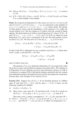

The document discusses tensor products of Hilbert spaces. It defines positive definite kernels on sets and shows how they can be used to define tensor products. Given Hilbert spaces H1, ..., Hn, it constructs a kernel on the cartesian product of the spaces and shows that its Gelfand pair (H,φ) gives a tensor product of the Hilbert spaces. The map φ from the product space into H is multilinear and H is the completion of the algebraic tensor product of the vector spaces H1, ..., Hn.


![[Vvedensky d.] group_theory,_problems_and_solution(book_fi.org)](https://cdn.slidesharecdn.com/ss_thumbnails/vvedenskyd-grouptheoryproblemsandsolutionbookfi-org-130405071812-phpapp02-thumbnail.jpg?width=640&height=640&fit=bounds)