Download as PDF, PPTX

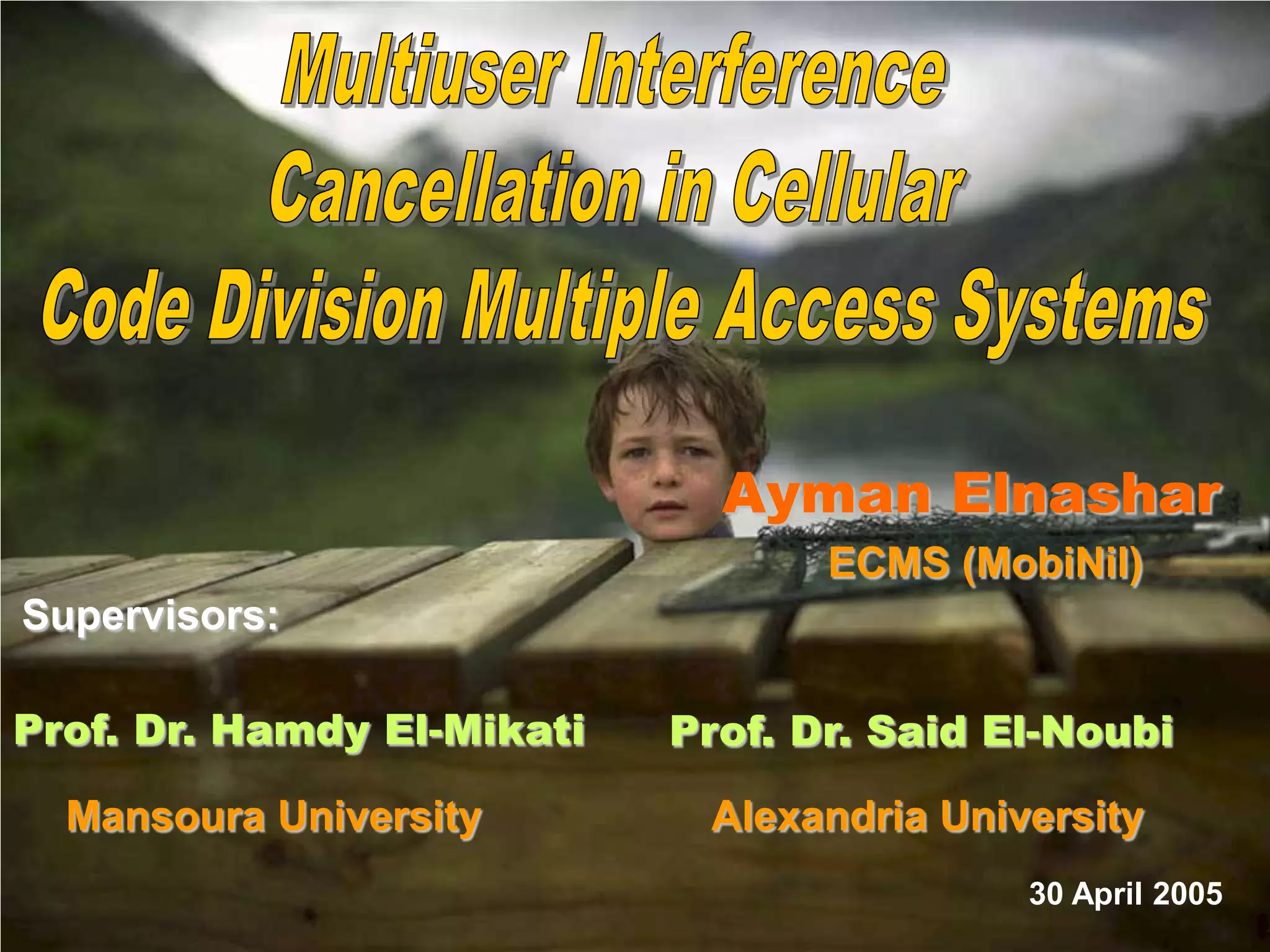
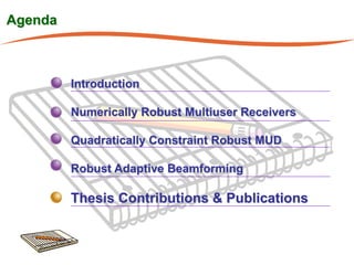
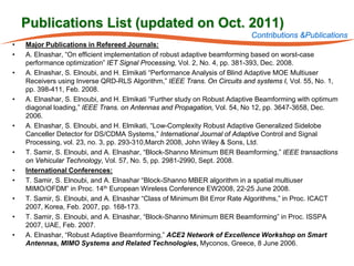
![Robust MOE with QI constraint (RSD-VL)
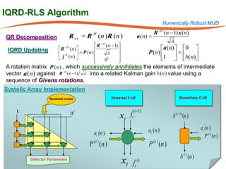
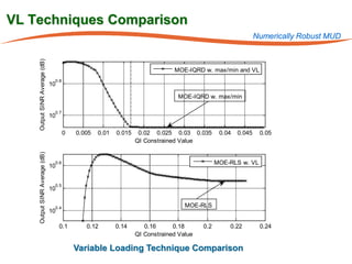
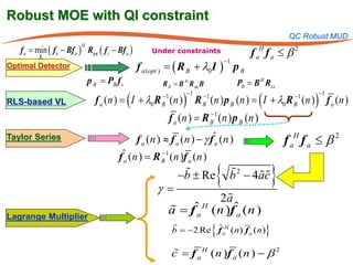
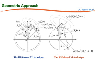
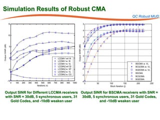
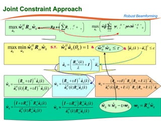
QC Robust MUD
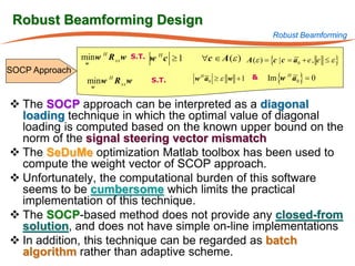
Ψ fa = f c − Bf a ) Rxx ( f c − Bf a ) + λ0 s ( f aH f a − β 2 )
1
(
H
Cost Function
2
Detector Update f a (n ) f a (n − 1) − µ∇f a (n )
=
Gradient Vector ∇f a (n ) = B H R xx (n )f c + B H R xx (n )Bf a (n − 1) + λ0f a (n − 1)
−
Robust Detector f a (n= f a (n − 1) − µ (R B (n )f a (n − 1) − p B (n )) − µλ0f a (n − 1)
)
Non-Robust f a (n= f a (n − 1) − µ [ R B (n )f a (n − 1) − p B (n )]
)
( ) ( )
H
QI Constraint f a (n ) − µλ0f a (n − 1) f a (n ) − µλ0f a (n − 1) ≤ β 2
Quadratic
Equation
2 H 2
0 { a 0 fa }
H (n) f (n − 1) λ + H (n) (n) − β 2 =
µ f a (n − 1) f a (n − 1)λ − 2µ Re f a fa 0
= µ 2 f a (n − 1)
2
a
−b ± b 2 − 4ac
Lagrange Multiplier λ0 =
2a
b =(n − 1)
f
H
{
−2µ Re a (n) f a }
(n ) 2 − β 2
= fa
c](https://image.slidesharecdn.com/phdpresentation-13198801469983-phpapp01-111029042616-phpapp01/85/Phd-Presentation-25-320.jpg)
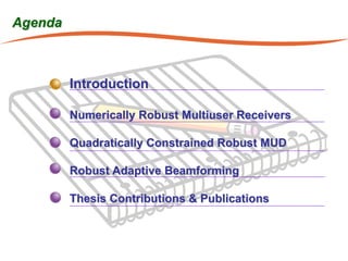
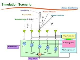
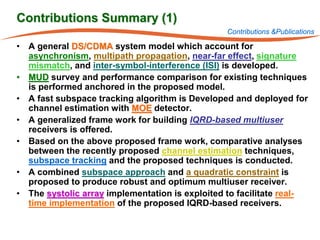
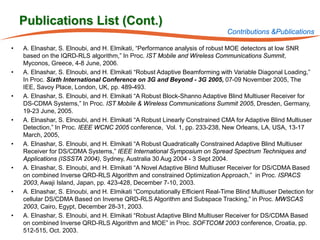
![Optimum Step-size of MOE-RSD w. VL
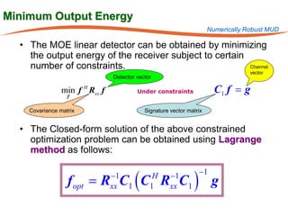
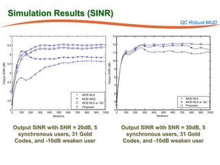
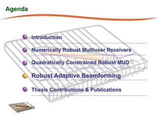
QC Robust MUD
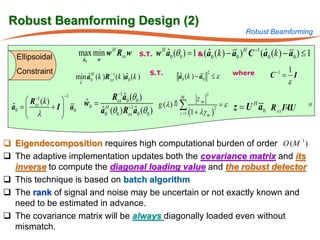
Ψ fa = f c − Bf a ) Rxx ( f c − Bf a ) + λ0 s ( f aH f a − β 2 )
1
(
H
Cost Function
2
Non-Robust Detector f a (n= f a (n − 1) − µ [ R B (n )f a (n − 1) − p B (n )]
)
( ) ( )
H
Updated Cost Function Ψ fa (n)
= f (n − 1) + µ B∇ fa (n) Rxx (n) f (n − 1) + µ B∇ fa (n)
Quadratic Equation
Ψ fa (= Ψ fa (n − 1) + 2µ (n)∇ Ha (n) PB f (n − 1) + µ 2 (n)∇ Ha (n) RB (n)∇ fa (n)
n)
f f
∂Ψ fa (n)
Differentiate =2∇ H (n) PB f (n − 1) + 2µ (n)∇ H (n) RB (n)∇ f (n)
f f zero
∂µ (n) a a a
2
α ∇ fa (n)
µopt (n) =
∇ H (n) RB (n)∇ f (n) + σ
fa a
Optimum Step-Size](https://image.slidesharecdn.com/phdpresentation-13198801469983-phpapp01-111029042616-phpapp01/85/Phd-Presentation-26-320.jpg)


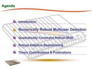
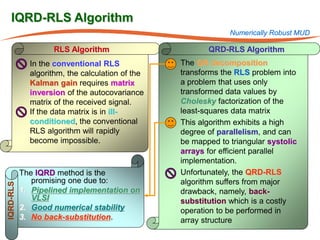
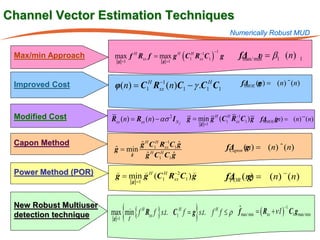
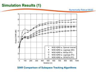
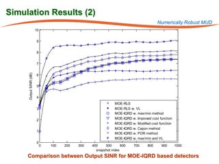
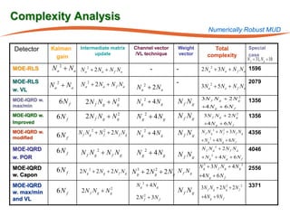
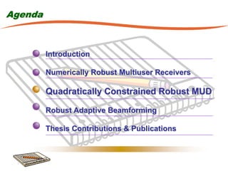
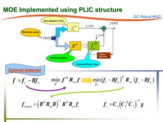
The document summarizes research on robust multiuser detection techniques for direct-sequence code-division multiple access (DS-CDMA) systems. It introduces numerically robust algorithms like the inverse QR decomposition RLS algorithm to overcome issues with conventional RLS algorithms in ill-conditioned environments. It also discusses the minimum output energy detector and its implementation using the IQRD-RLS algorithm. Finally, it outlines various channel estimation techniques used for multiuser detection like the max/min, improved cost, modified cost, Capon, and power methods.


