Automatic analysis and classification of surface electromyography

Frontiers Med. Biol. Engng, Vol. 11, No. 1, pp. 13–29 (2001)
Ó VSP 2001.
Original paper
Automatic analysis and classi cation of surface
electromyography
FATMA E. Z. ABOU-CHADI¤
, AYMAN NASHAR1
and MOHAMED SAAD2
1 Department of Electronics and Communications Engineering, Mansoura University, P.O. 35516,
Box 20, Mansoura, Egypt
2 Department of Neurology, Faculty of Medicine, Mansoura University, P.O. 35516, Box 20,
Mansoura, Egypt
Received 22 November 1999; revised 12 June 2000; accepted 22 August 2000
Abstract—In this paper, parametric modeling of surface electromyography (EMG) algorithms that
facilitates automatic SEMG feature extraction and arti cial neural networks (ANN) are combined
for providing an integrated system for the automatic analysis and diagnosis of myopathic disorders.
Three paradigms of ANN were investigated: the multilayer backpropagation algorithm, the self-
organizing feature map algorithm and a probabilistic neural network model. The performance of the
three classi ers was compared with that of the old Fisher linear discriminant (FLD) classi ers. The
results have shown that the three ANN models give higher performance. The percentage of correct
classi cation reaches 90%. Poorer diagnostic performance was obtained from the FLD classi er. The
system presented here indicates that surface EMG, when properly processed, can be used to provide
the physician with a diagnostic assist device.
Key words: Biological signal processing; surface electromyography;automatic classi cation; autore-
gressive modeling; neural networks.
1. INTRODUCTION
Electromyography (EMG) is the study of the electrical activity of muscle and forms
a valuable aid in the diagnosis of neuromuscular disorders. EMG ndings are
used to detect and describe different disease processes affecting the motor unit,
the smallest functional unit of the muscle. With voluntary muscle contraction, the
action potential re ecting the electrical activity of a single anatomical motor unit
can be recorded. It is the compound motor unit action potential (MUAP) of those
muscle bers within the recording range of the needle or surface electrodes [1].
¤
To whom correspondenceshould be addressed. E-mail: f-abochadi@ieee.org

14 F. E. Z. Abou-Chadi et al.
The MUAP waveform depends on the motor unit architecture, i.e. on the num-
ber of bers, their sizes and density, so the analysis of MUAP shape may provide
important information about the motor unit structure and its changes. The disease
processes which affect the structure and activity of the motor unit are re ected in
the changes of MUAP features, particularly those of the durations and amplitudes.
These changes may also manifest themselves as polyphasic potentials [2] charac-
terized by an increased number of phases and/or turns, i.e. in signals of a more
complicated shape than the normal MUAP. The changes of the MUAP shape are an
important indicator of motor unit disintegration and compensatory processes [3].
Recently, several authors successfully investigated muscle properties by analyzing
the time course of amplitude parameters, muscle ber conduction velocity and
spectral parameters of the EMG signal during voluntary and electrically elicited
isometric contractions [4, 5].
It is also well known and documented that the power spectral density function
of the EMG signal undergoes frequency compression during either voluntary or
electrically elicited sustained contractions [6], long before the muscle becomes
unable to produce the desired force. Such changes are referred to as myoelectric
manifestations of localized muscle fatigue.
The spectral content of the EMG signal depends on (i) the number of active
motor units whose electrical activity is sensed by the detection probe, (ii) their
ring rates, (iii) the position of the active muscle bers relative to the detection
probe and (iv) the velocity of propagation of depolarization along muscle bers [7].
During a sustained muscle contraction, the spectral compression is mainly due to
a progressive reduction of muscle ber conduction velocity and to the variation of
the spatial distribution of depolarization along the muscle bers [8]. Therefore, if
spectral parameters are studied, it is important to separate their random variations
due to estimation errors from those due to physiological events.
Previous approaches for analyzing the time-varying aspects of the EMG signals
have used a linear prediction model. Among them, the autoregressive (AR) model
has been used to deal with time-varying EMG signals because it emphasizes spectral
peaks for time records having a small number of samples [9]. This approach was
introduced by Graupe and Cline [10] who attempted to use the surface EMG signal
for controlling prostheses. Subsequently, Sherif et al. [11] studied the behavior
of AR integrated moving average (ARIMA) coef cients of the EMG signal from
the deltoid muscle during dynamic contractions. Capponi et al. [12] represented
EMG signals, detected from the biceps and triceps muscles, with the time courses
of AR coef cients during rapid isometric contractions. Recently, Kiryu et al. [13]
investigated the physiological interpretation of AR modeling. They analyzed the
time-varying behavior of AR parameters of well-conditioned EMG signals detected
during an isometric force-varying ramp contraction. The AR coef cients of the
EMG signal could be used as quantitative measures to monitor local muscle
fatigue [14, 15].

Classi cation of surface EMG 15
To further the development of quantitative EMG techniques, the need has emerged
for adding automated decision-making support to these techniques so that all data
is processed in an integrated environment. Towards this goal, Coatrieux et al. [16]
applied cluster analysis for the automatic diagnosis of pathology based on MUAP
records. Hassoun et al. [17] proposed automated EMG signal decomposition using
neural networks. Pattichis et al. [18] utilized arti cial neural networks (ANNs) for
the automatic classi cation of EMG features recorded using needle electrodes for
normal individuals and patients suffering from neuromuscular diseases. They used
seven features derived from the shape of the MUAP waveforms.
The main goal of the present work is threefold: to assure the usage of surface
EMG (SEMG) in clinical diagnosis, to characterize the SEMG signal through the
determination of the AR model parameters to be used for comparisons between
groups of patients or between an individual record and any population norms that
might become available, and to provide an ef cient classi cation for the different
pathological cases.
The classi cation approaches taken here are: the old Fisher linear discrimi-
nant (FLD) algorithm and three models of neural networks: the multilayer back-
propagation model, the self-organizing feature map (SOM) model and a probabilis-
tic neural network (PNN) model. A comparison of the performance of the four clas-
si ers is performed for normal individuals and patients suffering with myopathic
lesions.
2. DATA ACQUISITION
Twenty-eight subjects were used in this work: 14 normals and 14 suffering from
myopathy. SEMG signal was recorded from the deltoid muscle at 50% maximum
voluntary contraction (MVC) for 5 s using bipolar surface electrodes. The recording
points within the muscle are standardized. The Biopac data acquisition system
consists of an internal microprocessor MP100 data acquisition card with 16 analog
input channels connected to an Apple PC. The software used in data acquisition
is Acqknowledge version 2 software. Figure 1 illustrates examples of the SEMG
signals.
2.1. The sampling frequency
It is knownthat information exists in the EMG frequency spectrum up to frequencies
of 1 kHz, implying that in order to satisfy the Nyquist criterion, a sampling
frequency of at least 2 kHz would have to be used. However, for surface myoelectric
signals, most of the power in the signal is at low frequencies (below 300 Hz).
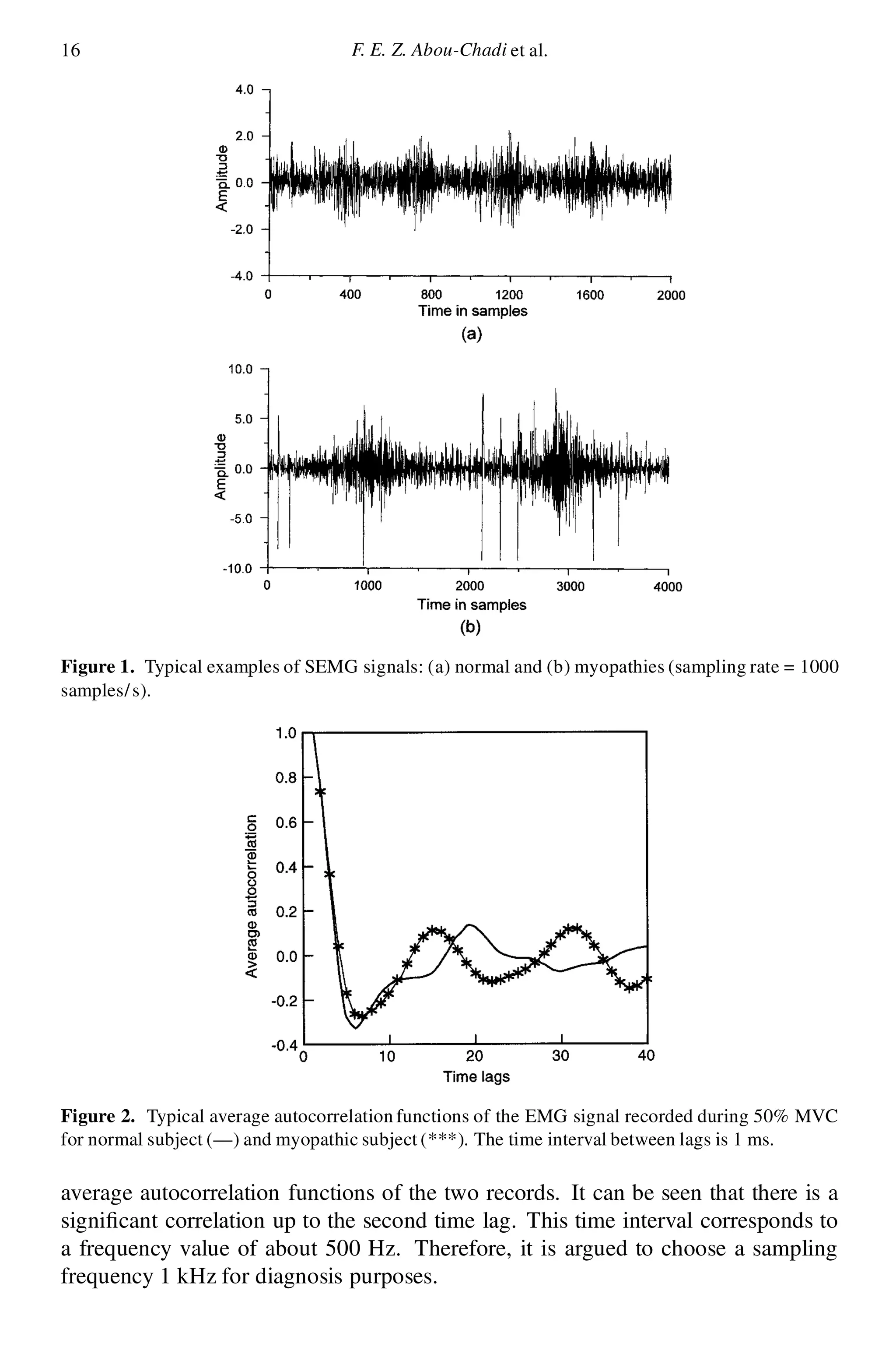
Further, consideration of average autocorrelation functions of the EMG recorded
in a myopathic subject and a normal subject taken from a pair of surface electrodes
placed over motor unit of the deltoid muscle indicates that the difference between
these functions is more pronounced at low frequencies. Figure 2 illustrates the

Figure 1. Typical examples of SEMG signals: (a) normal and (b) myopathies (sampling rate = 1000
samples/s).
Figure 2. Typical average autocorrelation functions of the EMG signal recorded during 50% MVC
for normal subject (—) and myopathic subject (***). The time interval between lags is 1 ms.
average autocorrelation functions of the two records. It can be seen that there is a
signi cant correlation up to the second time lag. This time interval corresponds to
a frequency value of about 500 Hz. Therefore, it is argued to choose a sampling
frequency 1 kHz for diagnosis purposes.

3. AR MODELING OF THE SEMG
In the AR model each sample emg(n) of the SEMG is described as a linear
combination of previous samples plus an error term e(n) that is independent of past
samples, i.e.
emg.n/ D ¡
pX
kD1
ak ¢ emg.n ¡ k/ C e.n/ (1)
where emg(n) is the output model signal, ak are the AR coef cients, e(n) is the
error sequence and p is the model order. The model represented by (1) can be used
in a backward fashion (retrospective regression analysis); the signal at time n is
considered as being the linear combination of p future values.
The system function is:
H .z/ D
1
1 C
pP
kD1
ak ¢ z¡k
(2)
H .z/ contains poles only. Thus, the model can work only for signals with a well-
de ned peaky spectrum and can be tted to SEMG. The spectrum of the sequence
emg(n) can be estimated from the model if we consider jE.!/j D 1 (white noise
sequence); therefore, the spectrum of the output signal is equal the spectrum of
H .z/ and can be estimated by substituting e¡j!
into z as follows:
S.!/ D jEMG.!/j2
D
1

1 C
pP
kD1
ak ¢ e¡j!k

2
(3)
The AR coef cients .ak/ are calculated using the covariance method [19] which
minimizes the residual energy
P
n e2
.n/.
3.1. Spectrum of the SEMG
The analysis was carried out on consecutive 500 ms segments of the EMG signal to
ensure the stationarity of the segment where SEMG was found to be stationary on a
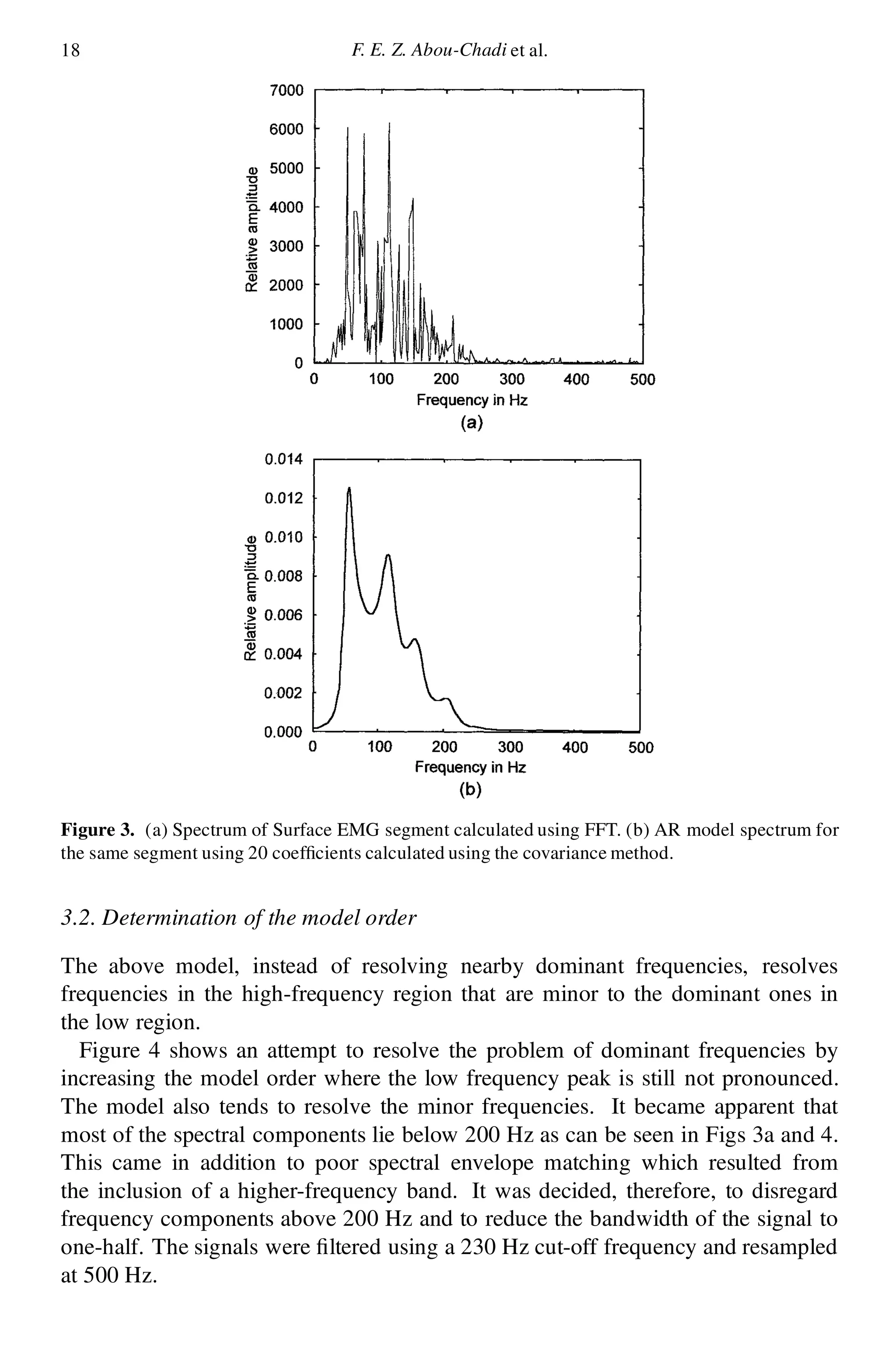
segment length of less than 0.64 s [8]. Figure 3a demonstrates the spectrum of such
segment calculated by a fast Fourier transform (FFT) routine. A consistent feature
of EMG spectra is the existence of many spectral peaks in the region 10–200 Hz.
The higher frequency regions, above 200 Hz, contain little minor amplitude
information compared to the lower frequency region. Figure 3b demonstrates the
spectrum of the AR model of the same signal calculated using 20 coef cients. It
can be seen here that instead of obtaining six dominant peaks, only three peaks
were obtained.

Figure 3. (a) Spectrum of Surface EMG segment calculated using FFT. (b) AR model spectrum for
the same segment using 20 coef cients calculated using the covariance method.
3.2. Determination of the model order
The above model, instead of resolving nearby dominant frequencies, resolves
frequencies in the high-frequency region that are minor to the dominant ones in
the low region.
Figure 4 shows an attempt to resolve the problem of dominant frequencies by
increasing the model order where the low frequency peak is still not pronounced.
The model also tends to resolve the minor frequencies. It became apparent that
most of the spectral components lie below 200 Hz as can be seen in Figs 3a and 4.
This came in addition to poor spectral envelope matching which resulted from
the inclusion of a higher-frequency band. It was decided, therefore, to disregard
frequency components above 200 Hz and to reduce the bandwidth of the signal to
one-half. The signals were ltered using a 230 Hz cut-off frequency and resampled
at 500 Hz.

Figure 4. AR model spectrum of Fig. 3a with 30 coef cients.
Figure 5. (a) The FFT spectrum of the EMG signal sampled at 500 Hz. (b) The AR model spectrum
of the same EMG segment with 20 coef cients calculated using the covariance method.

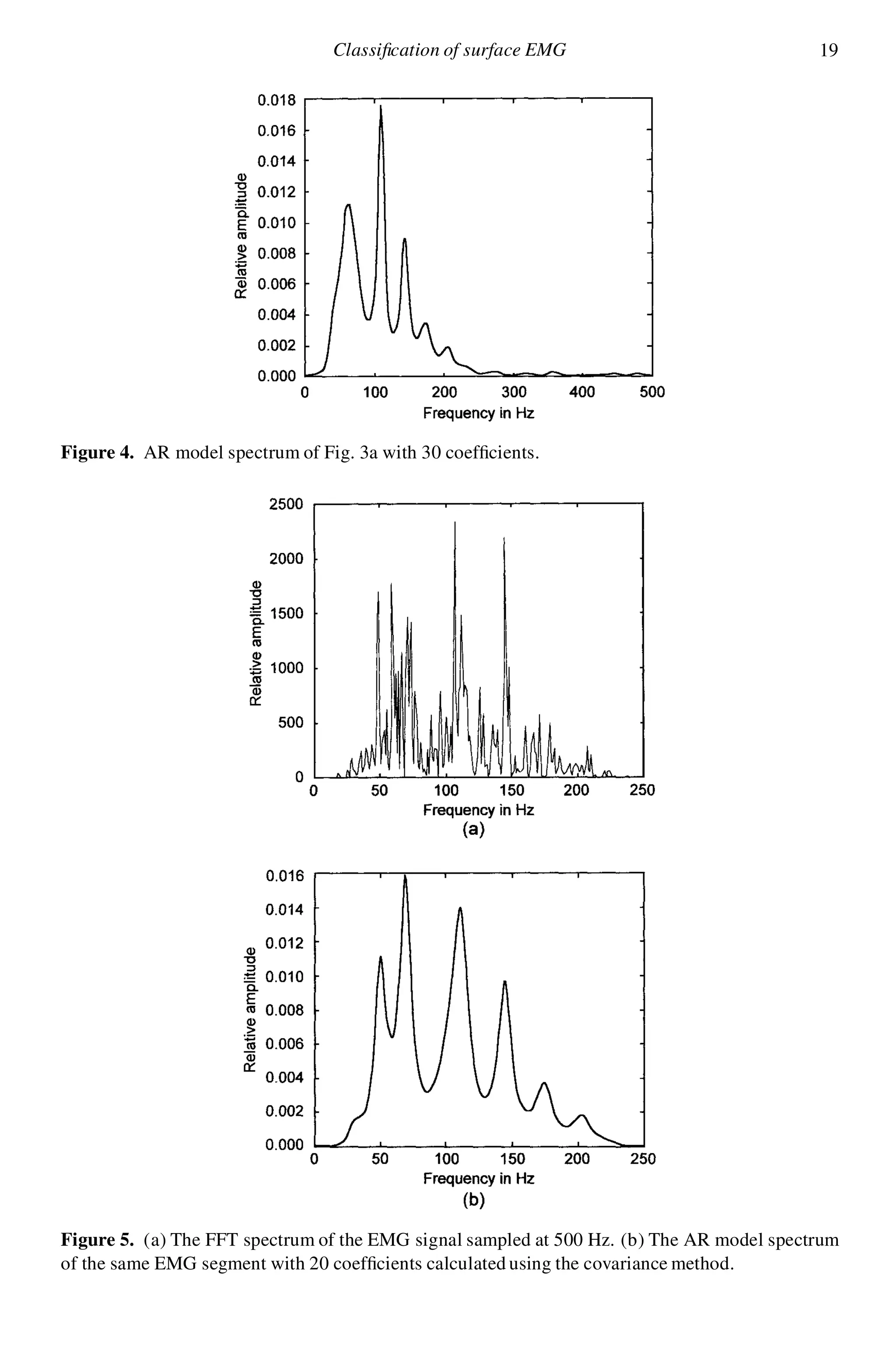
Figure 5a demonstrates the FFT spectrum of the ltered signal (230 Hz). Fig-
ure 5b illustrates the spectrum of the all-pole 20 coef cients model with the EMG
segment. It can be seen that most of the dominant frequencies are resolved and a
much better spectral envelope t is obtained. Therefore, a value of p D 20 was
chosen to characterize surface EMG segments as a compromise between model size
and accuracy of signal representation.
3.3. Determination of the number of segments
After characterizing each segment with 20 coef cients, it was observed from the
calculation of the spectra of consecutive segments that the spectrum changes from
segment to segment. Therefore, in order to determine how many segments would
be enough to fully describe each subject, the average value of each coef cient
was calculated and its convergence as a function of the number of segments was
investigated. It has been shown that the changes in the values of the AR parameters
become smaller after 10 segments. Therefore, it is argued to use 10 segments to
characterize each subject; each segment is 500 ms long.
4. CLASSIFICATION OF THE SEMG
The classi cation approaches taken here are: the old Fisher linear discriminant [20]
and ANN algorithms. Two paradigms for training the ANN are investigated,
i.e. supervised and unsupervised. For supervised learning, the well-known back-
propagation algorithm [21, 22], and for unsupervised learning, the SOM algo-
rithms [23, 24], have been implemented. A comparison of the performance of the
different classi ers is performed for normal and abnormal individuals. A training
group of nine normals and nine myopathies, and a test group of ve normals and
ve myopathies were used for ANN classi ers.
4.1. Fisher linear discriminant algorithm
The rst step in the classi cation procedure is the construction of the Fisher linear
discriminant vector (FLDV) W, where the two different classes =1 and =2 are
introduced as in the following equation [24]:
W D C¡1
t .¹1 ¡ ¹2/ (4)
where ¹1 and ¹2 are the means of the two classes =1 and =2, and Ct is the total
within-class covariance matrix de ned by
Ct D
X
n2=1
.Xn ¡ ¹1/ ¢ .Xn ¡ ¹1/T
C
X
n2=2
.Xn ¡ ¹2/ ¢ .Xn ¡ ¹2/T
After calculating the vector W, the projection of every subject that participates in
the construction of the vector is rst calculated and then the projection threshold

between the two different classes is determined. Using this threshold, the projection
of unknown subjects is found and classi ed in accordance with the above threshold.
It has been found that the results are dependent on the number of participants
in the construction of the FLDV. More participants mean better de nition of the
threshold between classes and thus better classi cation. Using nine normals and
nine abnormals to construct the FLDV, a 60% percent successful classi cation was
obtained for a test group of ve normals and ve abnormals.
4.2. Back-propagation neural network
The number of input nodes is 200 using the 20 AR coef cients for 10 SEMG
segments and the number of outputs is one output node, where the output is
corresponds to the two classes: normal and abnormal. The number of nodes in the
hidden layers is changed (3–10 nodes) in order to determine the optimum number
of nodes. A scaling method is used to scale the input patterns to give every pattern
the same importance.
The results of classi cation using the back-propagation neural network trained
with three different back-propagation algorithms are summarized in Tables 1–3.
ANN architectures with three layers (input layer, hidden layer and output layer)
were used [21, 22]. The ANN architectures are expressed as strings showing the
number of inputs, the number of nodes in the hidden layers and one output node.
The number of weights and the training time are tabulated for all models. During
the training phase, an error measure of the closeness of weights to a solution can
be calculated for each pattern (200 input features) that represents a subject in the
training set. This measure is used for determining whether a certain subject has
been learnt by the system and is de ned by:
PSS D .yl ¡ dl/2
(5)
where PSS is the Pattern sum squares, yl is the calculated output and dl is the desired
output. The PSS measure is then summed over all patterns (18 subjects) to get the
total sum of squares (TSS) measure:
TSS D
pX
nD1
.yl ¡ dl/2
n D 1; ¢ ¢ ¢ ; p (6)
where p is the number of training patterns (18 in this case; nine normals and nine
abnormals).
The average error EE estimated for the output node:
EE D .TSS=p/0:5
(7)
For comparing the results that were obtained by various classi cation algorithms,
common performance metrics have been used [19]. For a given decision suggested
by the output neuron, four possible alternatives exist: true positive (TP), false
positive (FP), true negative (TN) and false negative (FN). A TP decision occurs

when the positive diagnosis of the algorithm coincides with a positive diagnosis
according to the physician. A FP decision occurs when the algorithm made a
positive diagnosis that does not coincide the physician. A TN decision occurs when
the algorithm and the physician suggest the absence of a positive diagnosis. A FN
decision occurs when the algorithm made a negative diagnosis that does not agree
with the physician. From the above measures, correct classi cation percentage
(%CC) has been calculated for the N cases in the evaluation set:
%CC D 100 £ .TP C TN/=N (8)
Important issues that characterize the overall performance of the back-propagation
algorithms during the training procedure are:
(1) The output of all the back-propagation EMG models is limited between 1 and
0 range, so the selection of a sigmoidal activation function is preferred. The
hidden layer nodes activation functions were also set to a sigmoidal function.
(2) At present, no method other than empirical has been proposed for choosing the
architecture of feedforward neural networks so that for every training algorithm
three architectures were created and compared.
(3) Training all the neural network models is accomplished using batch training.
(4) Networks of Table 1 are trained using a variable learning rate algorithm [25].
The rst model architecture is insuf cient to generalize the network where
Training %CC D 100 but Evaluation %CC D 70. Models 2 and 3 are nearly
suitable for generalization of the network. If we attempt to move towards a
high architecture network, we will over t the data and the network will be less
generalized. The value of TSS will determine the generalization performance
of the network, i.e. a high EE value will lead to a high Training %CC but less
generalization where the network tends to memorize the training data; a small
EE value will lead to best generalization but may be less Training %CC.
(5) All models of Table 2 are trained using variable a learning rate algorithm
with an early stopping technique to determine the optimum value of EE. The
available records are subdivided into two sets: training set and validation set.
The problem of determining the suitable network architecture is removed using
this technique. The number of epochs is reduced using an early stopping
technique where the training will continue until validation test failure. In
training the networks there is not suf cient records to form an evaluation data
set, but with the rst two sets the basic idea of early stopping technique is
clari ed.
(6) Table 3 is a backpropagation model trained with the Conjugate Gradient
Algorithm [26]. Conjugate Gradient Training is faster than the old variable
learning rate algorithm and is more suitable to large size networks than other
fast algorithms. Therefore, it was found that it gives the highest performance
for the present application.

Table 1.
The results of EMG classi cation using neural network back-propagation trained with variable
learning rate
Model Architecture Weights Epochs EE Time
(s)
Training
%CC
Evaluation
%CC
1 200-3-1 603 323 10¡5 90 100 70
2 200-5-1 1005 328 10¡5 60 100 80
3 200-10-1 2010 285 10¡5 60 100 80
Table 2.
The results of EMG classi cation using neural network back-propagation trained with variable
learning rate (early stopping technique)
(s)
Training
%CC
Validation
%CC
1 200-3-1 603 188 0.0047 30 90 90
2 200-5-1 1005 118 0.0532 30 90 90
3 200-10-1 2010 148 0.0067 45 100 90
Table 3.
Results of classi cation using neural network back-propagation EMG models trained with the
conjugate gradient method and early stopping technique to improve generalization
(s)
Training
%CC
Validation
%CC
1 200-3-1 603 28 2.7 £ 10¡11
25 100 80
2 200-5-1 1005 18 3 £ 10¡6
20 100 90
3 200-10-1 2010 15 5.4 £ 10¡5
20 100 90
4.3. SOM
The neural network models in this system were derived using Kohonen’s SOM
algorithm [27]. The algorithm creates a map of relationships among input patterns.
The map is a reduced representation of the original data that preserves its topological
relationships, i.e. the map has fewer dimensions but the clusters keep their relative
positions. SOM creates the map from a random starting point without target results.
SOM output nodes do not correspond to known classes but to unknown clusters that
SOM nds in the data autonomously.
During the training process SOM nds the output node that has the least distance
from the training pattern. It then changes the node’s weights to increase its similarity
to the training pattern. It also changes the weights of a block of adjacent nodes even
though they have only random relationships to the training pattern. A wining neuron
(node) thus in uences its neighbors and different training patterns trigger different
winners with different neighbors. The overall effect is to move the output nodes to

Table 4.
Results of using SOM classi ers
Model No. of No. of Output ´ Epochs Time (s) Training Evaluation
Inputs Classes Grid %CC %CC
1 200 2 4 £ 4 0.9 1000 75 944 60
2 200 2 6 £ 6 0.9 1000 140 100 80
3 200 2 8 £ 8 0.9 1000 270 100 80
4 200 2 10 £ 10 0.9 1000 440 100 80
Figure 6. SOMs. (a) Maximum response map after training phase (100%). (b) Maximum response
with all nodes assigned.
‘positions’ that map the distribution of the training patterns. After training, each
node’s weights model the features that characterize a cluster in the data, i.e. SOM
nds natural clusters of feature similarities from unlabeled training data.
The results of the SOM models that were investigated with no preprocessing of
the 200 input feature vector are summarized in Table 4. Models with output grid
sizes (number of output nodes) of 4 £ 4, 6 £ 6, 8 £ 8 and 10 £ 10 were developed.
The initial gain factor ´ was selected to be 0.9. It has been suggested [27] that the
value of ´ should lie between 0 and 1, i.e. 0 < ´ < 1. Training for SOM EMG
models was carried out using 1000 epochs.
At each training cycle (epoch), the 18 training patterns were presented at random.
It was observed that grid sizes below 6 £ 6 were inadequate for producing models
with well-separated classes. All models succeed in classifying all patterns during
training phase, except for model 1.
The procedure that was followed for assigning normal and abnormal classes to the
SOM is presented here.
For every 200 element feature vector:
xn D x1;n; x2;n; ¢ ¢ ¢ ; x200;n
T
; n D 1; 2; ¢ ¢ ¢ ; p (9)
where p is the number of patterns in the training set (p D 18 patterns), there is
an output node at the grid for which maximum response Rmax is caused. This
node is assigned the class number of the vector (1 ! normal, 0 ! abnormal).
Figure 6a shows the nodes where maximum response was caused by the patterns in
the training set after the completion of the training phase.

Figure 7. SOMs. (a) Simpli ed map showing the two classes boundaries. (b) Maximum response
map for the evaluation set (%CC D 80).
Nodes with ‘£’ values have not been assigned to any class. For this model where
the output grid is 6 £ 6 (36 output nodes) with a training set of 18 patterns, at least
18 nodes will not be assigned to any pattern. This means that unknown patterns
falling on ‘£’ nodes will not be diagnosed.
During the next phase, the ‘£’ nodes are assigned to one of the classes as follows.
The data of each subject in the training set is applied at the input and the response
at a certain ‘£’ node is observed. The class of the subject that cause maximum
response at the node is assigned to the node. This procedure is applied for all
the ‘£’ nodes until all of them are assigned to a class as shown in Fig. 6b. Figure 7a
shows the two classes boundaries for all the nodes in the grid. Figure 7b shows the
grid after the evaluation phase using the test group: ve normal and ve abnormal
subjects which yield 80% correction classi cation (%CC).
The SOM system compared to the back-propagation neural network system has
the advantage of the results being presented pictorially, e.g. with this system one
can relate a certain patient with another patient, nd boundary cases and observe
the mapping of a patient over serial examinations. Training efforts for SOM models
was signi cantly reduced as compared to the back-propagation models.
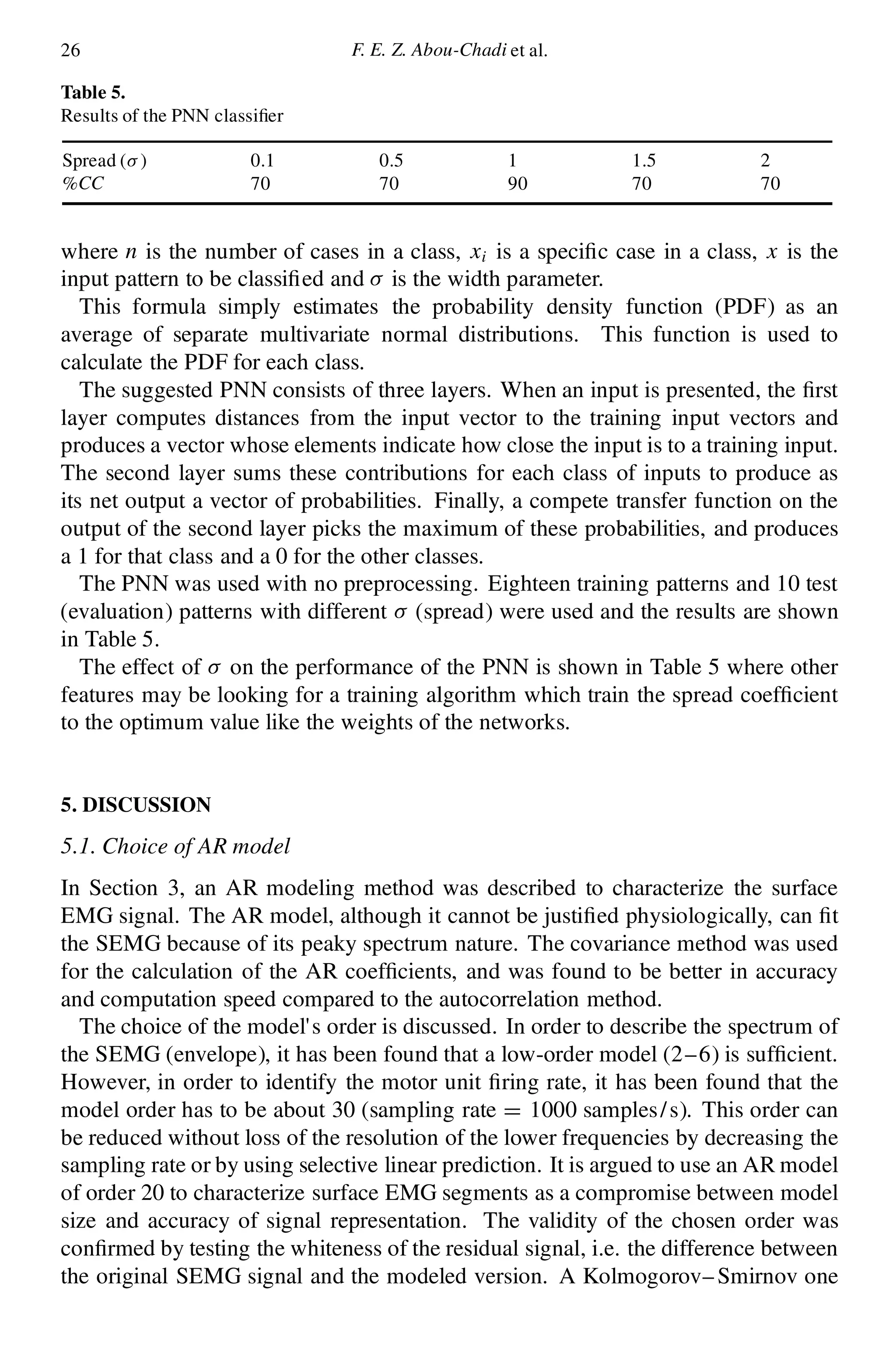
4.4. PNN
The PNN is a Bayesian classi er put into a neural network architecture [28, 29]. It
can be used as a function approximator like the back-propagation neural network.
The PNN should be used only for classi cation problems where there is a
representative training set. It can be trained quickly but has slow recall and is
memory intensive. It has solid underlying theory and can produce con dence
intervals. This network is simply a Baysian classi er put into a neural network
architecture. The PNN depends on the estimation of the probability density function
for every class using the Gaussian weighting function:
g.x/ D
1
n
nX
iD1
e
¡
kx¡xi k2
2¾ 2
(10)

Table 5.
Results of the PNN classi er
Spread (¾ ) 0.1 0.5 1 1.5 2
%CC 70 70 90 70 70
where n is the number of cases in a class, xi is a speci c case in a class, x is the
input pattern to be classi ed and ¾ is the width parameter.
This formula simply estimates the probability density function (PDF) as an
average of separate multivariate normal distributions. This function is used to
calculate the PDF for each class.
The suggested PNN consists of three layers. When an input is presented, the rst
layer computes distances from the input vector to the training input vectors and
produces a vector whose elements indicate how close the input is to a training input.
The second layer sums these contributions for each class of inputs to produce as
its net output a vector of probabilities. Finally, a compete transfer function on the
output of the second layer picks the maximum of these probabilities, and produces
a 1 for that class and a 0 for the other classes.
The PNN was used with no preprocessing. Eighteen training patterns and 10 test
(evaluation) patterns with different ¾ (spread) were used and the results are shown
in Table 5.
The effect of ¾ on the performance of the PNN is shown in Table 5 where other
features may be looking for a training algorithm which train the spread coef cient
to the optimum value like the weights of the networks.
5. DISCUSSION
5.1. Choice of AR model
In Section 3, an AR modeling method was described to characterize the surface
EMG signal. The AR model, although it cannot be justi ed physiologically, can t
the SEMG because of its peaky spectrum nature. The covariance method was used
for the calculation of the AR coef cients, and was found to be better in accuracy
and computation speed compared to the autocorrelation method.
The choice of the model’s order is discussed. In order to describe the spectrum of
the SEMG (envelope), it has been found that a low-order model (2–6) is suf cient.
However, in order to identify the motor unit ring rate, it has been found that the
model order has to be about 30 (sampling rate D 1000 samples/s). This order can
be reduced without loss of the resolution of the lower frequencies by decreasing the
sampling rate or by using selective linear prediction. It is argued to use an AR model
of order 20 to characterize surface EMG segments as a compromise between model
size and accuracy of signal representation. The validity of the chosen order was
con rmed by testing the whiteness of the residual signal, i.e. the difference between
the original SEMG signal and the modeled version. A Kolmogorov–Smirnov one

sample test [30] was used and the results showed that there was no signi cant
difference between the cumulative distributions of the two signals.
The SEMG was found to possess a changing spectral nature with a considerable
variance. To overcome this spectral variability and to determine how many segments
would be suf cient to fully describe each subject, the average value of each AR
was calculated and its convergence as a function of the number of segments was
investigated. The results showed that there was no change in the values of the
coef cients for 10 segments or more. Therefore, it is argued to use 10 segments
to characterize each subject, each segment is 500 ms long.
5.2. Classi cation
SEMG classi cation was performed using statistical and neural network classi ers.
Three paradigms of ANN were investigated: the multilayer back-propagation
algorithm, SOM algorithm and a PNN model. The performance of the three ANN
classi ers was compared with that of the old FLD classi er. The ANN techniques
performed better than the FLD and yielded a higher success rate. ANNs seem more
appropriate for the classi cation of SEMG because of their ability to adapt and to
create complex classi cation boundaries. The back-propagation neural networks
presented in this study performed well even with a limited amount of data and
achieved fast learning with a limited number of epochs. However, their performance
depends on the learning algorithm. Networks trained with the variable learning
rate method gives less percentage of correct classi cation than those trained using
other learning algorithms. A 90% correct classi cation has been achieved using the
conjugate gradient method or the early stopping technique.
The SOM investigated for the same real data required a much greater number of
learning epochs in order to converge and gave 80% correct classi cation. However,
SOM has the advantage of the results being presented pictorially. For example, one
can relate a certain patient with another patient, nd boundary cases and observe
the mapping of the patient over serial examinations. The PNN performed well but
its performance depends on the choice of the spread coef cient: a tuning procedure
must be used in order to achieve the best results.
Further developments to the adopted ANN methodologies may be easily achieved
by increasing the database used for training the neural networks and incorporating
other muscle diseases. This is the aim of the next stage of work.
6. CONCLUSIONS
An attempt to characterize the SEMG for clinical classi cation was made. It has
been demonstrated, that enough information remains in the recorded SEMG to allow
its usage in clinical classi cation. An AR model was selected to characterize the
signal since it reduces the dimensionality of spectral characterization.
ANN diagnosis models in conjunction with parametric analysis provide an
integrated solution to the problem of automated EMG evaluation. This approach is

very desirable because it minimizes observer bias, facilitates comparisons of results
across individual and different methodologies, and, more importantly, provides
useful information for helping the physician in reaching a more accurate diagnosis.
The system presented here indicates that the SEMG, when properly processed,
can replace needle EMG in some clinical applications and can be used to provide
the physician with a diagnostic assist device. The amount of data collected until
now is insuf cient for making signi cant conclusions concerning the accuracy of
classi cation. Yet it is suggested that the methods adopted have the potential of
becoming an effective diagnostic device. This is only the rst stage of a project
aiming at building an expert system for SEMG. Adding new cases and new types of
diseases seems to be the next and necessary steps.
REFERENCES
1. C. J. De Luca, Physiology and mathematics of myoelectric signals, IEEE Trans. BME-26,
313–325 (1979).
2. E. K. Rich eld, B. A. Cohen and J. W. Albers, Review of quantitative and automated needle
electromyographicanalyses, IEEE Trans. BME-28, 506–514 (1981).
3. J.-L. Coatrieux, On-line electromygraphic signal processing system, IEEE Trans. BME-31,
199–207 (1984).
4. K. C. McGill, K. L. Cummins and L. J. Dorfman, Automatic decomposition of the clinical
electromyogram, IEEE Trans. BME-32, 470–477 (1985).
5. E. A. Clancy and H. Hogan, Single site electromyography amplitude estimation, IEEE Trans.
BME-41, 159–167 (1994).
6. T. D’ Alessio, M. Kna itz, G. Balestra and S. Paggi, On-line estimation of myoelectric signal
spectral parameters and nonstationaritiesdetection, IEEE Trans. BME-40, 981–984 (1993).
7. F. Tanzi and V. Taglietti, Spectral analysis of surface motor unit action potentials and surface
interferenceelectromyogram,IEEE Trans. BME-28, 318–324 (1981).
8. G. F. Inbar and A. E. Noujaim, On surface EMG spectral characterizationand its application to
diagnostic classi cation, IEEE Trans. BME-31, 597–604 (1984).
9. T. Kiryu, Y. Saitoh and K. Ishioka, Investigation on parametric analysis of dynamics EMG
signals by a muscle-structuredsimulation model, IEEE Trans. BME-39, 280–288 (1992).
10. D. Graupe and W. K. Cline, Functional separation of SEMG signals via ARMA identi cation
methods for prosthesis control purpose, IEEE Trans. SMC-5, 252–259 (1975).
11. M. H. Sherif, R. J. Gregor and J. Lyman, Effects of load on myoelectric signals: The ARIMA
representation,IEEE Trans. BME-28, 411–416 (1981).
12. M. Capponi, T. D’ Alessio and M. Laurenti, Sequential estimation of power spectra for nonsta-
tionary myoelectric signals, Electromyogr. Clin. Neurophysiol.28, 427–432 (1988).
13. T. Kiryu, C. J. De Luca and Y. Saitoh, AR modeling of myoelectric interferencesignals during a
ramp contraction,IEEE Trans. BME-41, 1031–1038 (1994).
14. P. C. Doerschuk,D. E. Gustafon and A. S. Willsky, Upper extremitylimb functiondiscrimination
using EMG signal analysis, IEEE Trans. BME-30, 18–29 (1983).
15. G. Hefftner, W. Zucchini and G. G. Jaros, The electromyogram (EMG) as a control signal for
functional neuromuscular stimulation — Part II: practical demonstration of the EMG signature
discriminationsystem, IEEE Trans. BME-35, 238–242 (1988).
16. J. L. Coatrieux,P. Toulouse, B. Rouvrais and R. Le Bars, Automatic classi cation of electromyo-
graphic signals, EEG Clin. Neurophysiol.55, 333–341 (1983).

17. M. H. Hassoun, C. Wang and A. R. Spitzer, Neural network extraction of repetitive vectors for
electromyography.Part I and Part II, IEEE Trans. BME-41, 1039–1061 (1994).
18. C. S. Pattichis, C. N. Schizas and L. T. Middleton, Neural network models in EMG diagnosis,
IEEE Trans. BME-42, 468–496 (1995).
19. S. M. Kay, Modern Spectral Estimation. Prentice-Hall,Englewood Cliffs, NJ (1988).
20. R. Duda and P. Hart, Pattern Classi cation and Scene Analysis. Wiley Interscience, New York
(1975).
21. S. Haykin, Neural Networks: A Comprehensive Foundation. Prentice-Hall, Englewood Cliffs,
NJ (1998).
22. R. Beale and T. Jacson, Neural Computing: An Introduction. Adam Hilger, Bristol (1990).
23. T. Kohonen, The self-organizingmap, Proc. IEEE 78, 1464–1480 (1990).
24. R. Schalkoff, Pattern Recognition: Statistical, Structural and Neural Approaches. John Wiley,
New York (1992).
25. A. Cichocki and R. Unbehauen, Neural Networks for Optimization and Signal Processing. John
Wiley, New York (1993).
26. W. H. Hines, Matlab Supplement to Fuzzy and Neural Approaches in Engineering. John Wiley,
New York (1996).
27. J. Aleksander and H. Morton, An Introduction to Neural Computing. Chapman & Hall, London
(1992).
28. L. Streit Roy and T. X. Luginbuhl, Maximum likelihood training of probabilistic neural
networks, IEEE Trans. NN-5 (9) (1994).
29. D. F. Specht, Probabilistic neural networks and the polynomial adaline as complementary
techniques for classi cation, IEEE Trans. NN-1, 111–121 (1990).
30. S. Siegel, Nonparametric Statistics for Behavioral Sciences, McGraw-Hill, New York (1956).

Automatic analysis and classification of surface electromyography

More Related Content

What's hot

Viewers also liked

Similar to Automatic analysis and classification of surface electromyography

More from Dr. Ayman Elnashar, PhD

Recently uploaded

Automatic analysis and classification of surface electromyography