Download as PDF, PPTX

![Lemma I : multivariate Normal regression
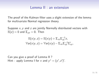
Suppose x and y are jointly Normally distributed vectors with
means E(x) and E(y ), respectively, with variance matrices Σxx and
Σyy , respectively, and covariance matrix Σxy . Then
−1
E(x|y ) = µx + Σxy Σyy (y − µy ),
Var(x|y ) = Σxx − Σxy Σyy Σ′ .
−1
xy
Define e = x − E(x|y ). Then
−1
Var(e) = Var([x − µx ] − Σxy Σyy [y − µy ])
= Σxx − Σxy Σyy Σ′
−1
xy
= Var(x|y ),
and
−1
Cov(e, y ) = Cov([x − µx ] − Σxy Σyy [y − µy ], y )
= Σxy − Σxy = 0.
14 / 35](https://image.slidesharecdn.com/paris2012session2-121108075413-phpapp01/85/Paris2012-session2-14-320.jpg)
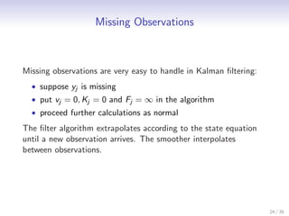
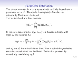

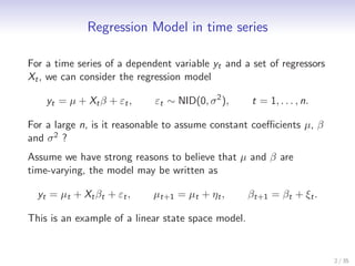
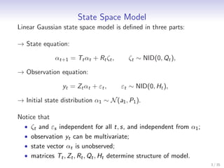
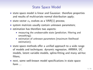
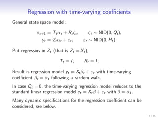
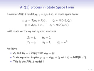
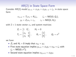
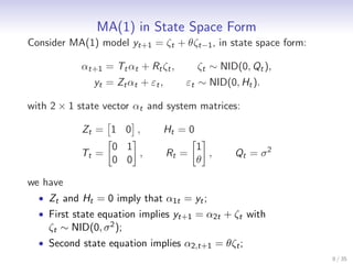
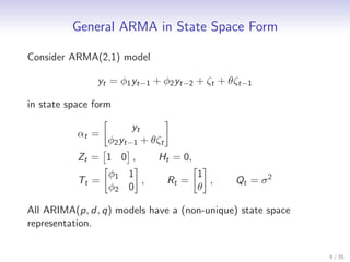
This document discusses state space methods for time series analysis and forecasting. It begins by introducing the basic state space model framework, which represents a time series using unobserved states that evolve over time according to a state equation and generate observations according to an observation equation. The document then provides examples of how various time series models, such as regression models with time-varying coefficients, ARMA models, and univariate component models can be expressed as state space models. Finally, it introduces the Kalman filter algorithm, which provides a recursive means of estimating the unobserved states from the observations.


![Lecture on nk [compatibility mode]](https://cdn.slidesharecdn.com/ss_thumbnails/lectureonnkcompatibilitymode-110825092241-phpapp01-thumbnail.jpg?width=640&height=640&fit=bounds)