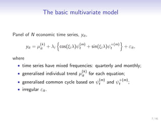
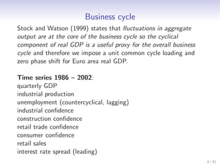
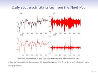
This document discusses time series forecasting and summarizes four illustrations of time series analysis and forecasting: 1. A multivariate model is used to analyze the European business cycle based on trends, common cycles, and leads/lags between economic indicators like GDP, industrial production, and confidence. 2. A bivariate unobserved components model is applied to daily Nordpool electricity spot prices and consumption data. The model decomposes the data into trends, seasons, cycles and residuals. Forecasting results show the bivariate model outperforms the univariate. 3. A periodic dynamic factor model is jointly modeled to 24 hours of French electricity load data. The model accounts for long-term trends, various seasonal patterns,

1. Time Series Forecasting
Siem Jan Koopman
http://personal.vu.nl/s.j.koopman
Department of Econometrics
VU University Amsterdam
Tinbergen Institute
2012

2. Unobserved components: decomposing time series
A basic model for representing a time series is the additive model
yt = µt + γt + εt , t = 1, . . . , n,
also known as the classical decomposition.
yt = observation,
µt = slowly changing component (trend),
γt = periodic component (seasonal),
εt = irregular component (disturbance).
In a Structural Time Series Model (STSM)
or a Unobserved Components Model (UCM),
the components are modelled explicitly as stochastic processes.
Basic example is the local level model.
2 / 91

3. Illustrations
We present various illustrations of time series analysis and
forecasting:
1. European business cycle
2. Bivariate analysis: decomposing and forecasting of Nordpool
daily (average) of spot prices and consumption.
3. Periodic dynamic factor analysis: joint modeling of 24 hours
in a daily panel of electricity loads.
4. Modelling house prices in Europe.
5. Modelling the U.S. Yield Curve.
3 / 91

4. Illustration 1: European business cycle
Azevedo, Koopman and Rua (JBES, 2006) consider European
business cycle based on
• a multivariate model consisting of generalised components for
trend and cycle with band-pass filter properties;
• data-set includes nine time series (quarterly, monthly) where
individual series that may be leading/lagging GDP;
• a model where all equations have individual trends but share
one common “business cycle” component.
• a common cycle that is allowed to shift for individual time
series using techniques developed by R¨nstler (2002).
u
4 / 91

5. Shifted cycles
0.2
0.0
−0.2
estimated cycles
gdp (red) versus
cons confidence (blue)
−0.4
1980 1985 1990 1995
0.2
0.0
−0.2
estimated cycles
gdp (red) versus
shifted cons confidence (blue)
−0.4
1980 1985 1990 1995
5 / 91

6. Shifted cycles
In standard case, cycle ψt is generated by
ψt+1 cos λ sin λ ψt κt
+ =φ + +
ψt+1 − sin λ cos λ ψt κ+
t
The cycle
+
cos(ξλ)ψt + sin(ξλ)ψt ,
is shifted ξ time periods to the right (when ξ > 0) or to the left
(when ξ < 0).
Here, − 1 π < ξ0 λ < 2 π (shift is wrt ψt ).
2
1
More details in R¨nstler (2002) for idea of shifting cycles in
u
multivariate unobserved components time series model of
Harvey and Koopman (1997).
6 / 91

7. The basic multivariate model
Panel of N economic time series, yit ,
(k) (m) +(m)
yit = µit + λi cos(ξi λ)ψt + sin(ξi λ)ψt + εit ,
where
• time series have mixed frequencies: quarterly and monthly;
(k)
• generalised individual trend µit for each equation;
(m) +(m)
• generalised common cycle based on ψt and ψt ;
• irregular εit .
7 / 91

8. Business cycle
Stock and Watson (1999) states that fluctuations in aggregate
output are at the core of the business cycle so the cyclical
component of real GDP is a useful proxy for the overall business
cycle and therefore we impose a unit common cycle loading and
zero phase shift for Euro area real GDP.
Time series 1986 – 2002:
quarterly GDP
industrial production
unemployment (countercyclical, lagging)
industrial confidence
construction confidence
retail trade confidence
consumer confidence
retail sales
interest rate spread (leading)
8 / 91

9. Eurozone Economic Indicators
14.30 GDP Retail sales
IPI unemployment
Interest rate spread Industrial confidence indicator
14.25 Construction confidence indicator Retail trade confidence indicator
Consumer confidence indicator
14.20
14.15
14.10
14.05
14.00
13.95
13.90
1990 1995 2000
9 / 91

10. Details of model, estimation
• we have set m = 2 and k = 6 for generalised components
• leads to estimated trend/cycle estimates with band-pass
properties, Baxter and King (1999).
• frequency cycle is fixed at λ = 0.06545 (96 months, 8 years),
see Stock and Watson (1999) for the U.S. and ECB (2001)
for the Euro area
• shifts ξi are estimated
• number of parameters for each equation is four (σi2,ζ , λi , ξi ,
σi2,ε ) and for the common cycle is two (φ and σκ )
2
• total number is 4N = 4 × 9 = 36
10 / 91

11. Decomposition of real GDP
14.2 0.003
14.1
0.002
14.0
0.001
GDP Euro Area Trend slope
13.9
1990 1995 2000 1990 1995 2000
0.01 0.0050
0.0025
0.00
0.0000
−0.0025
−0.01
−0.0050
Cycle irregular
1990 1995 2000 1990 1995 2000
11 / 91

12. The business cycle coincident indicator
Selected estimation results
series load shift R2d
gdp −− −− 0.31
indutrial prod 1.18 6.85 0.67
Unemployment −0.42 −15.9 0.78
industriual c 2.46 7.84 0.47
construction c 0.77 1.86 0.51
retail sales c 0.26 −0.22 0.67
consumer c 1.12 3.76 0.33
retail sales 0.11 −4.70 0.86
int rate spr 0.57 16.8 0.22
12 / 91

13. Coincident indicator for Euro area business cycle
0.010
0.005
0.000
−0.005
−0.010
−0.015
1990 1995 2000
13 / 91

14. Coincident indicator for growth
• tracking economic activity growth is done by growth indicator
• we compare it with EuroCOIN indicator
• EuroCOIN is based on generalised dynamic factor model of
Forni, Hallin, Lippi and Reichlin (2000, 2004)
• it resorts to a dataset of almost thousand series referring to
six major Euro area countries
• we were able to get a quite similar outcome with a less
involved approach by any standard
14 / 91

15. EuroCOIN and our growth indicator
0.0150
0.0125
0.0100
0.0075
0.0050
0.0025
0.0000
−0.0025
−0.0050
−0.0075 Coincident Eurocoin
1990 1995 2000
15 / 91

16. Illustration 2: Nord Pool data
• we consider Norwegian electricity prices and consumption
from Nord Pool.
• mostly hydroelectric power stations; supply depends on
weather.
• Norway’s yearly hydro power plant capacity is 115 Tw hours.
• Nord Pool is day ahead market: daily trades for next day
delivery.
• daily series of average of 24 hourly price and consumption.
• spot prices measured in Norwegian Kroner (8 NOK ≈ 1 Euro).
• sample: Jan 4, 1993 to April 10, 2005; 640 weeks or 4480
days.
• data are subject to yearly cycles, weekly patterns, level
changes, and jumps.
16 / 91

17. Bivariate analysis: daily spot prices and consumption
Our unobserved components model is given by
2
yt = µt + γt + ψt + xt′ λ + εt , εt ∼ NID(0, σε ),
where
• yt is bivariate: electricity spot price and load consumption;
• µt is long term level;
• γt is seasonal effect with S = 7 (day of week effect);
• ψt is yearly cycle changes (summer/winter effects);
′
• xt λ has regression effects, mainly dummies for special days;
• εt is the irregular noise.
Parameter estimation and forecasting of observations have been
carried out by the STAMP 8 program of Koopman, Harvey,
Doornik and Shephard (2008, stamp-software.com):
user-friendly but still flexible, also for multivariate models.
17 / 91

18. Daily spot electricity prices from the Nord Pool
(i) (ii)
0.1
6
0.0
5
4 −0.1
3
−0.2
100 200 300 400 500 600 100 200 300 400 500 600
(iii) (iv)
0.50
1
0.25
0
0.00
−1
−0.25
100 200 300 400 500 600 100 200 300 400 500 600
Univariate decomposition of Nord Pool daily prices January 4, 1993 to April 10, 2005:
(i) data and estimated trend plus regression; (ii) seasonal component (S = 7, the day-of-week effect); (iii) yearly
cycle; (iv) irregular.
18 / 91

19. Joint decomposition of electricity prices & consumption
7
(i−a) 0.50
(i−b)
6 0.25
0.00
5 −0.25
450 500 550 600 450 500 550 600
(ii−a) 0.010
(ii−b)
0.05 0.005
0.000
−0.05
−0.005
450 500 550 600 450 500 550 600
(iii−a) 0.50
(iii−b)
1 0.25
0.00
0
−0.25
450 500 550 600 450 500 550 600
(iv−a) (iv−b)
0.2 0.025
0.0
−0.025
−0.2
450 500 550 600 450 500 550 600
Bivariate decomposition of prices and consumption: Feb 19, 2001 to April 10, 2005:
(ia,b) data and estimated trend plus regression; (iia,b) seasonal component (S = 7, the day-of-week effect); (iiia,b)
yearly cycle; (iva,b) irregular.
19 / 91

20. Forecasting results
We present MAPE for forecasting of one- to seven-days ahead prices for both uni- and bivariate models. The one-
to seven-days ahead forecasts are for the next seven days. The first forecast is for Monday, March 14, 2005 in
Week 637. The last forecast is for Sunday, April 10, 2005 in Week 640. The weeks 638 and 639 contain calendar
effects for Maundy Thursday (March 24, 2005) and the days until Easter Monday (March 28, 2005).
week 637 week 638 week 639 week 640
uni biv uni biv uni biv uni biv
horizon
1M 0.83 1.11 0.15 0.07 0.83 1.01 0.92 0.27
2T 0.86 0.94 0.51 0.53 1.20 1.36 0.74 0.20
3W 1.43 1.55 0.67 0.79 1.40 1.52 0.62 0.16
4T 1.94 2.09 0.64 0.88 1.71 1.75 0.60 0.14
5F 1.69 1.93 0.65 0.72 2.01 2.00 0.60 0.30
6S 1.62 1.95 0.58 0.69 2.26 2.17 0.67 0.43
7S 1.61 2.05 0.68 0.90 2.44 2.27 0.79 0.56
20 / 91

21. Illustration 3: periodic dynamic factor analysis
Aim: the joint modeling of 24 hours in a daily panel of electricity
loads for EDF.
Focus: modelling and short-term forecasting of hourly electricity
loads, from one day ahead to one week ahead.
• EDF provides a long time series: 9 years of hourly loads
• We can establish a long-term trend component but also
• different levels of seasonality (yearly, weekly, daily)
• special day effects (EJP)
• weather dependence (temperature, cloud cover)
• We look at the intra-year as well as the long-run dynamics by
using these different components.
21 / 91

22. Periodic dynamic factor model specification
The adopted methodology builds on Dordonnat, et al (2008, IJF):
• Model is for high-frequency data, for hourly data);
• Hours are in the cross-section (yt is 24 × 1 vector);
• The model dynamics are formulated for days: a multivariate
daily time series model;
• In effect, we adopt a periodic approach to time series
modelling;
• The right-hand side of the model is set-up as a multiple
regression model;
• We let the regression parameters evolve over time (days);
• We have a time-varying regression model, written in
state-space form;
• The 24-dimensional time-varying parameters are subject to
common dynamics (random walks);
• Novelty: dynamic factors in the time-varying parameters.
22 / 91

23. Daily National Electricity Load, 1995-2004
80000
80000
National Load (MegaWatts)
National Load (MegaWatts)
60000
60000
40000
40000
2000 2005 2002 2003
Year (a) Date (b)
80000
50000
National Load (MegaWatts)
National Load (MegaWatts)
60000
40000
40000
30000
0 5 10 15 20 −5 0 5 10 15 20 25 30
Days elapsed since August 8th,2004 (c) National Temperature (°C) (d)
Time series and temperature effects at 9 AM
23 / 91

24. Daily National Electricity Load, 1995-2004
60000
60000
Mean Load (MegaWatts)
Mean Load (MegaWatts)
50000
50000
40000
40000
1 2 3 4 5 6 7 8 9 10 11 12 4 8 12 16 20 24
60000
60000
Month (a) Hour (b)
Mean Load (MegaWatts)
Mean Load (MegaWatts)
50000
50000
40000
40000
4 8 12 16 20 24 4 8 12 16 20 24
Hour (c) Hour (d)
Average patterns
(c) Oct-Mar, (d) Apr-Sep
24 / 91

25. Multivariate Time Series Model
A periodic approach: from a univariate hourly to a daily 24 × 1
vector:
yt = (y1,t . . . yS,t )′ , S = 24 hours per day, t = 1, . . . , T days.
Our multivariate time-varying parameter regression model is given
by:
K
yt = µ t + Btk xtk + εt , εt ∼ IIN (0, Σε ) , t = 1, . . . , T ,
k=1
• Trends: µt = (µ1,t . . . µS,t )′
k k k
• Daily vectors of explanatory variables xt = (x1,t . . . xS,t )′ ,
k = 1, . . . , K , depending only on the day or on the hour of the
day.
k k k
• Regression coefficients βt = (β1,t . . . βS,t )′ , k = 1, . . . , K . In
matrix form: Bt k = diag (β k ), k = 1, . . . , K
t
• Irregular Gaussian white noise εt = (ε1,t . . . εS,t )′ .
25 / 91

26. Time-varying regressions and dynamic factors
K
yt = µ t + Btk xtk + εt , εt ∼ IIN (0, Σε ) , t = 1, . . . , T ,
k=1
where the time-varying regression parameters are given by
µt = c 0 + Λ0 ft0 ,
k
βt = c k + Λk ftk , k = 1, . . . , K , t = 1, . . . , T ,
j j
with constant c j = (c1 . . . cS )′ , S × R j factor loading matrices Λj
and R j dynamic factors ftj = (f1,t . . . fR j ,t )′ , for j = 0, . . . , K and
j j
0 ≤ R j ≤ S.
• Factor structure requires 0 < R j < S;
• Constant parameter component for R j = 0;
• Model has unrestricted component when R j = S;
• Identification restrictions apply.
26 / 91

27. Dynamic factor specfications
Local linear trend model for factors in trends µt :
ft+1 = ftj
j
+ gtj + v jt , v jt ∼ IIN(0, Σj )
v
j
gt+1 = gtj + w jt , w jt ∼ IIN(0, Σj )
w
• vector of dynamic factors ftj ,
• slope or gradient vector gtj ,
• level disturbance v jt and slope disturbance w jt .
Random walk model for factors in the regression coefficients:
ft+1 = ftj + e jt ,
j
e jt ∼ IIN(0, Σe ),
j
j = 1, . . . , K , t = 1, . . . , T ,
with regression coefficient disturbance e jt .
27 / 91

28. Empirical application to French national hourly Loads
• French national hourly electricity loads from Sept-95 until
Aug-04
• Estimation of trivariate models for neighbouring hours
• Smooth trends
• Intentional missing values for special days (EJP) and turn of
the year. No problem for state space models.
• Yearly pattern regressors: sine/cosine functions of time are
used (2 frequencies)
• Day-of-the-week effects: day-type dummy regressors
• Weather dependence: heating degrees, smoothed-heating
degrees and cloud cover
• Heating degrees beneath treshold temperature of 15 C
• Exponentially smoothed temperature
• Cooling degrees above treshold temperature of 18 C
• Implemention: SsfPack 3 of Koopman, Shephard and
Doornik (2008, ssfpack.com) for Ox 6 (2008, doornik.com)
28 / 91

29. Yearly pattern estimates per hour
4 ˆk k
µs,t +
ˆ k=1 βs,t xs,t for hours (a) s = 0, 1, 2 ; (b) s = 3, 4, 5 ; (c) s = 6, 7, 8 (with extra component), etc.
Estimation: Jan 1997 - Aug 2003, Graph: Jan 1998 - Aug 2003.
29 / 91

30. Components 9 AM, factor model (blue) and univariate
Factor Univariate
1500 Factor Univariate
500 1000
0 500
2000 (a) 2002 2000 (b) 2002
300 Factor Univariate
−500 Factor Univariate
200 −1000
100 −1500
2000 (c) 2002 2000 (d) 2002
0 Factor Univariate
−6000 Factor Univariate
−8000
−200
−10000
2000 (e) 2002 2000 (f) 2002
−10000 Factor Univariate
60000 Factor Univariate
−12500
50000
−15000
2000 (g) 2002 2000 (h) 2002
ˆ9
(a) heating β9,t , (b) smoothed-heating, (c) cooling, (d) Monday, (e) Friday, (f) Saturday, (g) Sunday, (h) trend +
yearly pattern
30 / 91

31. 9 AM st. errors, factor model (blue) and univariate
Factor Univariate Factor Univariate
300 500
200
250
100
2000 (a) 2002 2000 (b) 2002
75 Factor Univariate
300 Factor Univariate
50 200
25 100
2000 (c) 2002 2000 (d) 2002
80 Factor Univariate 500 Factor Univariate
70
60 300
50
2000 (e) 2002 2000 (f) 2002
750 Factor Univariate
2000 Factor Univariate
500
1000
250
2000 (g) 2002 2000 (h) 2005
ˆ9
(a) heating s.e. β9,t , (b) smoothed-heating, (c) cooling, (d) Monday, (e) Friday, (f) Saturday, (g) Sunday, (h)
trend + yearly pattern
31 / 91

32. Sample ACFs of residuals (daily lags)
0.2 0.2 0.2 0.2
0.0 0.0 0.0 0.0
0 100 200 300 0 100 200 300 0 100 200 300 0 100 200 300
0.2 0.2 0.2 0.2
0.0 0.0 0.0 0.0
0 100 200 300 0 100 200 300 0 100 200 300 0 100 200 300
0.2 0.2 0.2 0.2
0.0 0.0 0.0 0.0
0 100 200 300 0 100 200 300 0 100 200 300 0 100 200 300
0.2 0.2 0.2 0.2
0.0 0.0 0.0 0.0
0 100 200 300 0 100 200 300 0 100 200 300 0 100 200 300
0.2 0.2 0.2 0.2
0.0 0.0 0.0 0.0
0 100 200 300 0 100 200 300 0 100 200 300 0 100 200 300
0.2 0.2 0.2 0.2
0.0 0.0 0.0 0.0
0 100 200 300 0 100 200 300 0 100 200 300 0 100 200 300
Selecting the right model requires experience and stamina!
32 / 91

33. Conclusions
• A general, flexible and insightful methodology is developed.
• Many dynamic features of load and price data can be
captured.
• We can detect many interesting signals which are not
discovered before.
• Decent forecasts.
• Decent diagnostics.
• Many possible extensions.
• Remaining challenge: a full multivariate unobserved
components model for all 24 hours to capture evolutions of
complete intradaily load pattern.
• More work is required !
33 / 91

34. Short Bibliography
• “Multivariate structural time series models” by Harvey and
Koopman (1997), Chapter in Heij et al. (1997) Wiley.
• “Time-series analysis by state-space methods” by Durbin and
Koopman (Oxford, 2001)
• “Periodic Seasonal Reg-ARFIMA-GARCH Models for Daily
Electricity Spot Prices” by Koopman, Ooms and Carnero
(JASA, 2007).
• “An hourly periodic state-space for modelling French national
electricity load” by Dordonnat, et.al. (International Journal of
Forecasting, 2008)
• “Forecasting economic time series using unobserved
components time series models” by Koopman and Ooms
(2011), Chapter in Clements and Hendry, OUP Handbook of
Forecasting.
34 / 91

35. Illustration 4: The macroeconomy in the euro area
Quarterly time series, 1981 – 2008, GDP in volumes,
for countries (i) France, (ii) Germany, (iii) Italy and (iv) Spain.
(i) (ii)
13.2
12.8
13.0
12.6
12.8
12.4
1980 1985 1990 1995 2000 2005 2010 1980 1985 1990 1995 2000 2005 2010
12.7 (iii) 12.25 (iv)
12.6
12.00
12.5
11.75
12.4
12.3 11.50
1980 1985 1990 1995 2000 2005 2010 1980 1985 1990 1995 2000 2005 2010
35 / 91

36. Illustration 4: The housing market in the euro area
Quarterly time series, 1981 – 2008, real house prices (HP),
for countries (i) France, (ii) Germany, (iii) Italy and (iv) Spain.
(i) 0.3 (ii)
5.0
0.2
4.5 0.1
4.0 0.0
1980 1985 1990 1995 2000 2005 2010 1980 1985 1990 1995 2000 2005 2010
(iii) (iv)
3.0
0.25
0.00 2.5
−0.25 2.0
1980 1985 1990 1995 2000 2005 2010 1980 1985 1990 1995 2000 2005 2010
36 / 91

37. Any (common) cyclical dynamics in the data ?
Autocorrelograms and sample spectra, based on first differences...
GDP−Correlogram GDP−Spectrum HP−Correlogram HP−Spectrum
1 1
(i) 0.4 0.4
0 0
0.2 0.2
0 10 20 0.0 0.5 1.0 0 10 20 0.0 0.5 1.0
1 1 0.75
(ii) 0.2
0.50
0 0
0.1 0.25
0 10 20 0.0 0.5 1.0 0 10 20 0.0 0.5 1.0
1 1
(iii) 0.4 0.50
0 0
0.2 0.25
0 10 20 0.0 0.5 1.0 0 10 20 0.0 0.5 1.0
1 1
(iv) 0.4 1.0
0 0
0.2 0.5
0 10 20 0.0 0.5 1.0 0 10 20 0.0 0.5 1.0
37 / 91

38. The basic multivariate model
Multiple set of M economic time series, yit , is collected in
yt = (y1t , . . . , yMt )′ and model is given by
(1) (2)
yt = µt + ψt + ψt + εt ,
where the disturbance driving each vector component is a vector
too, with a variance matrix. The structure of the variance matrix
determines the dynamic interrelationships between the M time
series.
For example, if trend component µt follows the random walk,
µt+1 = µt + ηt with disturbance vector ηt , with variance matrix
Ση :
• diagonal Ση , independent trends;
• rank(Ση ) = p < M, common trends (cointegration);
• rank(Ση ) = 1, single underlying trend;
• Ση is zero matrix, constant.
Similar considerations apply to other components.
38 / 91

39. Dynamic factor representations
We can formulate the multivariate unobserved components model
also by
(1) (2)
yt = µ∗ + Aη µt + A(1) ψt
κ + A(2) ψt
κ + Aε εt ,
where, for the trend component, for example, the loading matrix
Aη is such that
′
Ση = Aη Aη ,
and, similarly, loading matrices are defined for the other variance
matrices of disturbances that drive the components.
(1) (2)
Here the dynamic factors or unobserved components µt , ψt , ψt
and εt are ”normalised”.
39 / 91

40. STAMP
Model is effectively a state space model: Kalman filter methods
can be applied for maximum likelihood estimation of parameters
(such as the loading matrices).
Kalman filter methods are employed for the evaluation of the
likelihood function and score vector.
Kalman filter and smoothing methods are employed for signal
extraction or the estimation of the unobserved components.
User-friendly software is available for state space analysis.
We have used S T A M P for this research project: a
multi-platform, user-friendly software: econometrics, time series
and forecasting by clicking.
It can treat multivariate unobserved components time series
models...
40 / 91

41. Motivation of our study
• Evidence of any relationship between housing prices and GDP
in the euro area.
• Focus on more recent developments...
• We prefer to model the time series jointly and establish
interrelationships between the time series
• Focus on cyclical dynamics, long-term and short-term
• Emphasis on real housing prices: relevant for the monetary
policy
• We also like to discuss synchronisation of housing markets in
euro area
Empirical results are based on our data-set with two variables:
GDP and real house prices (HP); and for four euro area countries:
France, Germany, Italy and Spain.
41 / 91

42. Relevant literature
• Unobserved components model: Harvey (1989)
• State space methods: Durbin and Koopman (2001)
• Multivariate unobserved components: Harvey and Koopman
(1997), Azevedo, Koopman and Rua (2006);
• Parametric approaches for house prices:
• Probit regressions: Borio and McGuire, 2004, van den Noord,
2006;
• Dynamic Factor models: Terrones, 2004, DelNegro and Otrok,
2007, Stock and Watson, 2008;
• VAR: Vargas-Silva, 2008, Goodheart and Hofmann, 2008.
42 / 91

43. Univariate analysis
Objectives:
• Verify the trend-cycle decomposition for each series
• Verify whether possible restrictions are realistic
Results for GDP:
• two short cycles in France and Italy are detected (¡6 years);
• Germany and Spain contain both a short cycle (5.42 and 3.62
years, resp.) and a long cycle (13.5 and 9.11 years)
• Various cycles are deterministic (fixed sine-cosine wave)
Results for HP:
• Results are quite different for each series
• Two cycles for Germany (5.4 and 13.5 years)
• Two short cycles for Italy (3.0 and 5.5 years) and France (3.1
and 5.8 years)
• For Spain a cycle reduces to an AR(1) process
43 / 91

44. Univariate results for GDP
France Germany Italy Spain
GDP R R R R
Trend var 0.65 0.03 0.01 0.03 0.48 0.03 0.10 0.03
Cycle 1 var 0.81 0.17 0.00 0.15 3.85 5.75 0.07 0.00
Cycle 1 ρ 0.94 0.90 1.0 0.90 0.87 0.90 0.95 0.90
Cycle 1 p 3.04 5 5.42 5 2.97 5 3.62 5
Cycle 2 var 0.00 1 1.81 2.86 0.00 7.79 0.00 2.31
Cycle 2 ρ 1.0 0.95 0.95 0.95 1.00 0.95 1.00 0.95
Cycle 2 p 5.8 12 13.5 12 5.50 12 9.11 12
Irreg var 1 0.0 1 1 1 1 1 1
N 7.2 11.4 3.23 5.23 6.58 11.1 27.1 34.9
Q 14.5 24.9 15.1 14.6 9.26 13.3 22.1 24.8
R2 0.31 0.24 0.11 0.02 0.23 0.12 0.22 0.12
44 / 91

45. Univariate results for HP
France Germany Italy Spain
RHP R R R R
Trend var 0.59 0.03 0.34 0.03 0.00 0.03 0.39 0.03
Cycle 1 var 0.00 0.01 0.31 1.51 0.04 0.02 1 0.01
Cycle 1 ρ 1.0 0.90 0.97 0.90 0.96 0.90 0.34 0.90
Cycle 1 p 6.34 5 4.48 5 1.11 5 – 5
Cycle 2 var 0.00 2.19 1 19.9 1 49.4 0.00 39.5
Cycle 2 ρ 1.0 0.95 0.61 0.95 0.99 0.95 0.99 0.95
Cycle 2 p 8.37 12 2.82 12 13.3 12 – 12
Irreg var 1 1 0 1 0 1 0 1
N 23.8 0.59 5.89 9.95 7.03 8.32 36.1 11.9
Q 10.6 187 55.5 111 13.7 68.4 29.3 127
R2 0.61 0.25 0.35 0.15 0.56 0.22 0.47 0.28
45 / 91

46. Cycle correlations from univariate analysis
(1) (2)
Correlations for combined cycles (ψt + ψt ):
• Strong correlations between GDP of four countries
(correlations range from 0.52 to 0.94)
• The correlations with German GDP are the lowest
• Correlations between HP of four countries range from 0.42 to
0.94
• The highest correlation is between Spain and France HP’s
• Correlation on combined cycle are mostly due to long-term
cycle, not to the short-term cycle
• Correlations between GDP and HP for each country range
from 0.06 for Germany to 0.76 for Spain
• Overall low cross-correlations between GDP of one country
and HP of another country
46 / 91

47. Correlations between combined cycles for eight series
(1) (2)
Combined cycle (ψt + ψt )
F GDP F HP G GDP G HP I GDP I HP S GDP S HP
F GDP 1.00 0.51 0.52 0.23 0.83 0.15 0.89 0.61
F HP 0.51 1.00 0.44 0.44 0.52 0.68 0.68 0.94
G GDP 0.52 0.44 1.00 0.50 0.54 0.47 0.61 0.44
G HP 0.23 0.44 0.50 1.00 0.08 0.80 0.22 0.42
I GDP 0.83 0.52 0.54 0.08 1.00 0.06 0.84 0.64
I HP 0.15 0.68 0.47 0.80 0.06 1.00 0.29 0.64
S GDP 0.89 0.68 0.61 0.22 0.84 0.29 1.00 0.76
S HP 0.61 0.94 0.44 0.42 0.64 0.64 0.76 1.00
47 / 91

48. Correlations between short cycle for eight series
(1)
Short cycle ψt
F GDP F HP G GDP G HP I GDP I HP S GDP S HP
F GDP 1.00 0.46 0.40 0.24 0.64 -0.46 0.57 0.42
F HP 0.46 1.00 0.29 0.62 0.33 -0.51 0.35 0.39
G GDP 0.40 0.29 1.00 0.32 0.75 -0.16 0.67 0.58
G HP 0.24 0.62 0.32 1.00 0.18 -0.52 0.06 0.13
I GDP 0.64 0.33 0.75 0.18 1.00 -0.13 0.61 0.65
I HP -0.46 -0.51 -0.16 -0.52 -0.13 1.00 -0.25 -0.19
S GDP 0.57 0.35 0.67 0.06 0.61 -0.25 1.00 0.75
S HP 0.42 0.39 0.58 0.13 0.65 -0.19 0.75 1.00
48 / 91

49. Correlations between long cycle for eight series
(2)
Long cycle ψt
F GDP F HP G GDP G HP I GDP I HP S GDP S HP
F GDP 1.00 0.51 0.53 0.23 0.89 0.16 0.90 0.63
F HP 0.51 1.00 0.46 0.44 0.58 0.68 0.68 0.94
G GDP 0.53 0.46 1.00 0.52 0.44 0.49 0.62 0.46
G HP 0.23 0.44 0.52 1.00 0.07 0.82 0.22 0.43
I GDP 0.89 0.58 0.44 0.07 1.00 0.08 0.90 0.72
I HP 0.16 0.68 0.49 0.82 0.08 1.00 0.29 0.64
S GDP 0.90 0.68 0.62 0.22 0.90 0.29 1.00 0.76
S HP 0.63 0.94 0.46 0.43 0.72 0.64 0.76 1.00
49 / 91

50. Bivariate analysis
For each country, we carry out a bivariate analysis between GDP
and RHP:
(1) (2)
yt = µt + ψt + ψt + εt ,
where yt is a 2 × 1 vector for two series: GDP and HP.
We can conclude that
• highest correlation is found for cycle components (except
Italy)
• for France, high correlation for medium-term cycle (8 years)
but no dependence for long-term cycle (15.6 years)
• for Spain, strong correlations for both medium-term (8.2
years) and long-term (14.4 years)
• for Germany, correlations for both cycles, but with low periods
(4.3 and 7 years)
50 / 91

51. Bivariate results for GDP and HP
GDP RHP corr per ρ diag GDP RHP
FRA
trend 0.0 0.0 0.0 – – N 3.25 13.4
cyc 1 3.0 3.3 0.88 8.0 0.98 Q 17.0 17.4
cyc 2 1.0 126 0.07 15.6 0.99 R2 0.38 0.63
irreg 0.6 1.6 -0.19 – –
GER
trend 0.0 0.003 0.0 – – N 8.52 1.08
cyc 1 2.5 5.4 -0.6 4.3 0.90 Q 6.86 42.1
cyc 2 3.1 0.5 1.0 7.0 0.98 R2 0.39 0.29
irreg 4.3 1.1 0.58 – –
51 / 91

52. Bivariate results for GDP and HP
GDP RHP corr per ρ diag GDP RHP
ITA
trend 0.1 0.9 -0.15 – – N 4.19 4.57
cyc 1 4.3 16.2 -0.08 6.0 0.92 Q 10.1 8.60
cyc 2 0.0 8.4 0.0 1.1 0.94 R2 0.14 0.47
irreg 0.8 1.2 0.96 – –
SPN
trend 0.0 0.0 0.0 – – N 9.05 21.7
cyc 1 3.3 11.9 0.95 8.2 0.98 Q 17.5 43.0
cyc 2 0.0 83.3 0.82 14.4 0.99 R2 0.45 0.73
irreg 3.9 7.7 -0.35 – –
52 / 91

53. Four-variate cross-country analysis of GDP and RHP
Now we incorporate earlier findings and impose a strict short- and
long-term cycle decomposition for our analysis.
In particular, we have
• an independent trend µt (i.e. diagonal variance matrix Ση for
disturbance vectors of µt+1 = µy + ηt )
• similarly, an independent irregular component εt (i.e. diagonal
variance matrix Σε )
• a two-cycle parametrization with restricted periods of 5 and
12 years
• the rank of the 4 × 4 cycle variance matrices Σκ is 2:
common cyles ...
• we load the two ”independent” cycles on France and Germany,
i.e. cyclical dynamics of Spain and Italy are obtained as linear
functions of the two times two (short and long) cyclical factors
53 / 91

54. Four-variate decomposition for GDP, cross-country
13.00 LFRA_GDP Level LGER_GDP Level LITA_GDP Level
12.25 LSPA_GDP Level
13.25 12.6
12.75 12.00
13.00 11.75
12.50 12.4
12.75 11.50
1980 1990 2000 2010 1980 1990 2000 2010 1980 1990 2000 2010 1980 1990 2000 2010
LFRA_GDP−Cycle 1 LGER_GDP−Cycle 1
0.02 LITA_GDP−Cycle 1
0.010 LSPA_GDP−Cycle 1
0.01 0.02 0.01 0.005
0.00 0.00 0.00 0.000
−0.01 −0.02 −0.01 −0.005
1980 1990 2000 2010 1980 1990 2000 2010 1980 1990 2000 2010 1980 1990 2000 2010
LFRA_GDP−Cycle 2 LGER_GDP−Cycle 2 LITA_GDP−Cycle 2
0.050 LSPA_GDP−Cycle 2
0.025 0.025 0.02 0.025
0.000 0.000 0.000
0.00
−0.025 −0.025 −0.025
1980 1990 2000 2010 1980 1990 2000 2010 1980 1990 2000 2010 1980 1990 2000 2010
LFRA_GDP−Irregular LGER_GDP−Irregular
0.0050 LITA_GDP−Irregular
0.02 LSPA_GDP−Irregular
0.001 0.01
0.0025 0.01
0.000 0.00 0.0000 0.00
−0.001 −0.01 −0.0025 −0.01
1980 1990 2000 2010 1980 1990 2000 2010 1980 1990 2000 2010 1980 1990 2000 2010
54 / 91

55. Four-variate results for cross-country: GDP
Fra Ger Ita Spn Fra Ger
Cycle short (cov ×10−6 ) factor loadings
Fra 4.11 0.25 ∗ 0.77 ∗ -0.40 ∗ 1 0
Ger 1.77 11.8 0.81 ∗ 0.78 ∗ 0 1
Ita 5.65 10.1 13.1 0.27 ∗ 1.08 0.69
Spn -1.04 3.50 1.27 1.65 -0.41 0.35
Cycle long (cov ×10−6 )
Fra 8.08 0.79 ∗ 0.48 ∗ 0.98 ∗ 1 0
Ger 7.94 12.5 -0.16 ∗ 0.64 ∗ 0 1
Ita 3.43 -1.39 6.28 0.66 ∗ 1.42 -1.02
Spn 11.2 9.11 6.73 16.4 1.79 -0.41
55 / 91

56. Four-variate results for cross-country: GDP
• Diagnostic statistics are satisfactory
• Strong correlation France-Germany for long-term cycle
• Business cycles for Italy and Spain are closely connected with
the one for France (however, negative ??? marginal
correlation Fra-Spa for short-term cycle)
• German cycles strongly affect business cycles in Italy and
Spain (however, their marginal correlations for longer cycle are
negative)
56 / 91

57. Four-variate decomposition for HP, cross-country
5.5 LFRA_RHprice Level
0.3 LGER_RHprice Level LITA_RHprice Level LSPA_RHprice Level
0.25 3.0
5.0 0.2
4.5 0.00 2.5
0.1
4.0 −0.25 2.0
0.0
1980 1990 2000 2010 1980 1990 2000 2010 1980 1990 2000 2010 1980 1990 2000 2010
0.02 LFRA_RHprice−Cycle 1
0.02 LGER_RHprice−Cycle 1 LITA_RHprice−Cycle 1
0.04 LSPA_RHprice−Cycle 1
0.01 0.05 0.02
0.00
0.00 0.00
0.00
−0.02 −0.01
−0.02
1980 1990 2000 2010 1980 1990 2000 2010 1980 1990 2000 2010 1980 1990 2000 2010
LFRA_RHprice−Cycle 2
0.050 LGER_RHprice−Cycle 2
0.2 LITA_RHprice−Cycle 2 LSPA_RHprice−Cycle 2
0.1 0.1 0.2
0.025
0.0 0.000 0.0 0.0
−0.1 −0.1 −0.2
−0.025
1980 1990 2000 2010 1980 1990 2000 2010 1980 1990 2000 2010 1980 1990 2000 2010
LFRA_RHprice−Irregular LGER_RHprice−Irregular
0.002 LITA_RHprice−Irregular LSPA_RHprice−Irregular
0.01 5e−5 0.01
0.001
0.00 0 0.000 0.00
−0.01 −5e−5 −0.001
1980 1990 2000 2010 1980 1990 2000 2010 1980 1990 2000 2010 1980 1990 2000 2010
57 / 91

58. Four-variate results for cross-country: HP
Fra Ger Ita Spn Fra Ger
Cycle short (cov ×10−6 ) factor loadings
Fra 15.5 0.37 ∗ -0.89 ∗ 0.05 ∗ 1 0
Ger 4.73 10.8 0.10 ∗ -0.91 ∗ 0 1
Ita -21.0 1.97 36.2 -0.50 ∗ -1.64 0.90
Spn 0.89 -14.6 -14.6 23.8 0.55 -1.60
Cycle long (cov ×10−6 )
Fra 44.5 0.38 ∗ 0.70 ∗ 0.93 ∗ 1 0
Ger 4.43 3.13 -0.40 ∗ 0.69 ∗ 0 1
Ita 66.9 -10.3 207.1 0.38 ∗ 2.13 -6.30
Spn 100.4 19.9 88.3 262.8 1.89 3.69
58 / 91

59. Four-variate results for cross-country: HP
• Overall, these results seem to indicate that there is less
evidence of common (cyclical) dynamics in HP series
• Low correlations between France and Germany
• Strong negative correlations for the 5-year cycle between
Fra-Ita and Ger-Spa
• However, more commonalities for the 12-year cycle (Fra-Spa,
Fra-Ita, Ger-Spa)
• Similarities between correlation matrices for the 12-year HP
and GDP cycles, except that relationship Fra-Ger is stronger
for GDP (0.79 against 0.38 for HP)
59 / 91

60. Eight-variate results: HP and GDP for four countries
Similar restrictions apply as in four-variate analyses.
We conclude that
• strong correlations among GDPs for short-term cycles but less
evidence for long-term cycles, especially for Germany
• low correlations among HP series.
• for short-term cycle, these correlations for HP Fra-Ger is 0.65
and for HP Spa-Ger is -0.95.
• only a few positive correlations for the long-term cycle in HP
have been found: Fra-Spa (0.58) and Ger-Ita (0.57)
• correlations HP-GDP are only found for long-term cycle,
especially for France and Spain.
60 / 91

61. Eight-variate results: short cycle correlations
France Germany Italy Spain
GDP HP GDP HP GDP HP GDP HP
F-G 1 -0.33 0.67 0.10 0.81 -0.59 0.77 0.13
F-H 1 0.075 0.65 -0.35 -0.13 -0.12 -0.64
G-G 1 0.17 0.80 -0.27 0.88 -0.011
G-H 1 0.055 -0.26 -0.10 -0.95
I-G 1 -0.037 0.66 0.034
I-H 1 -0.55 -0.040
S-G 1 0.34
S-H 1
61 / 91

62. Eight-variate results: long cycle correlations
France Germany Italy Spain
GDP HP GDP HP GDP HP GDP HP
F-G 1 0.95 0.19 0.043 0.72 0.41 0.54 0.50
F-H 1 0.44 0.24 0.63 0.43 0.57 0.58
G-G 1 0.41 -0.31 0.26 0.44 0.21
G-H 1 -0.005 0.57 0.036 0.29
I-G 1 0.045 0.12 0.37
I-H 1 0.13 0.099
S-G 1 0.61
S-H 1
62 / 91

63. Illustration 5 : Modelling U.S. Yield Curve
Yield (in %)
6.50
6.25
6.00
5.75
5.50
5.25
Maturity (in months)
0 10 20 30 40 50 60 70 80 90 100 110 120
63 / 91

64. Time Series of Four Maturities
Yield (in %) Time to maturity: 3 month
10 Yield (in %) Time to maturity: 1 year
8
8
6
6
4
4
Date Date
1985 1990 1995 2000 1985 1990 1995 2000
Yield (in %) Yield (in %)
Time to maturity: 3 year Time to maturity: 10 year
10
10.0
8
7.5
6
5.0
Date Date
1985 1990 1995 2000 1985 1990 1995 2000
64 / 91

65. Term Structure of Interest Rates over Time
10.0
Yield (Percent)
7.5
5.0
125
100
75 2000.0
Mat 1997.5
urity 50 1995.0
(Mo
nths 1992.5
) 25 1990.0 Time
1987.5
65 / 91

66. Literature Review
Earlier analyses of this data:
• Affine Term Structure Models (ATSM):
Vasicek (1977), Cox, Ingersoll, and Ross (1985), Duffie and
Kan (1996), Dai and Singleton (2000), and De Jong (2000)
• Nelson-Siegel Model (NS):
Nelson and Siegel (1987), Diebold and Li (2006), Diebold,
Rudebusch and Aruoba (2006), De Pooter (2007), and
Koopman, Mallee, and Van der Wel (2009)
• Arbitrage-Free Nelson-Siegel Model (AFNS):
Christensen, Diebold, and Rudebusch (2007)
• Functional Signal plus Noise (FSN):
Bowsher and Meeks (2008)
In all cases: a dynamic factor model set-up !
66 / 91

67. Still Some Outstanding Issues...
• Which of these models provides an accurate description of the
data?
• Duffee (2002) and Bams and Schotman (2003) provide
evidence against affine term structure models
• What are the dynamics of the underlying factors:
Stationary or Nonstationary?
• Stationary: Affine Term Structure Models, Nelson-Siegel,
Arbitrage-Free Nelson-Siegel
• Nonstationary: Campbell and Shiller (1987), Hall, Anderson
and Granger (1992), Engsted and Tanggaard (1994) and
Bowsher and Meeks (2008)
• What are the dynamics of the underlying factors: #lags?
• Almost all models take a VAR(1) for the factor dynamics
• Exception: Bowsher and Meeks (2008)
67 / 91

68. Further Outline
• (General) Dynamic Factor Model (DFM)
• General Set-Up
• Stationary and Nonstationary
• Smooth Dynamic Factor Model (SDFM)
• Specification
• Knot Selection
• Other Restrictions of the DFM
• Results
• Conclusion
68 / 91

69. The Dynamic Factor Model (DFM)
• Time series panel of N monthly yield observations
yt = (yt (τ1 ), . . . , yt (τN ))′ with yt (τi ) the yield at time t with
maturity τi
• The general dynamic factor model is given by:
yt = µy + Λft + εt , εt ∼ N(0, H),
ft = Uαt
αt+1 = µα + T αt + R ηt , ηt ∼ N(0, Q),
for t = 1, . . . , n
• In here ft is an r -dimensional stochastic process that is
generated by the p-dimensional state vector αt and ηt is a
q × 1 vector
• We take H diagonal and have for the p × 1 initial state
α1 ∼ N(a1 , P1 ), and assume N >> r , r ≤ p and p ≥ q
69 / 91

70. The Dynamic Factor Model (DFM) – Cont’d
• Vectors µy and µα , and matrices Λ, H, U, T and Q are
system matrices, R is selection matrix of ones and zeros
• Special case of state space model.
• All vector autoregressive moving average processes can be
formulated in this framework (see, e.g., Box, Jenkins and
Reinsel (1994))
• In this paper: VAR and Cointegrated VAR (CVAR) for ft .
Obtained by suitable specification of U, T and R
• Elements of system matrices µy , Λ, H, µα , T and Q generally
contain parameters that need to be estimated
70 / 91

71. The Dynamic Factor Model (DFM) – Cont’d
• Need to impose restrictions on loading and variance matrices
to ensure identification, see Jungbacker and Koopman (2008):
• Vectors µy and µα not both estimated without restrictions
=¿ Restrict µα = 0 to focus on loading matrix Λ
• Impose restrictions on Λ, T & Q that govern covariances
=¿ Restrict r rows in Λ to be r × r identity matrix:
 
1 0 0
 0 1 0 
 
 0 0 1 
 
Λ =  λ4,1 λ4,2 λ4,3 
 
 . . .
. . 
. 
 . . .
λN,1 λN,2 λN,3
71 / 91

72. Dynamic Factor Model (DFM) – Stationary Case
• Take a VAR(k) model for the r × 1 vector ft :
k−1
ft+1 = Γt−j ft−j + ζt , ζt ∼ NID(0, Qζ )
j=0
• Stationarity imposed by restriction that |Γ(z)| = 0 has all
roots outside the unit circle
• Can write this ft in DFM. For example, for k = 1 have
αt = ft ,
U = Ir ,
R = Ir ,
T = Γ0 ,
Q = Qζ
72 / 91

73. Dynamic Factor Model (DFM) – Nonstationary Case
• Now the ft are generated by a cointegrated vector
autoregressive process:
k−1
∆ft+1 = βγ ′ ft + Γj ∆ft−j + ζt , ζt ∼ N(0, Qζ ),
j=0
• The r × s matrices β and γ have full column rank; in the
nonstationary case s < r and all ft nonstationary
• We propose an alternative but observationally equivalent
specification for ft via factor rotation:
f¯N ′
f¯ = t
= β⊥ γ ft ,
t
f¯S
t
¯
also need to construct new loading matrix Λ = ¯
ΛN ¯
ΛS
73 / 91

74. Dynamic Factor Model (DFM) – Estimation
• As noted earlier, the Dynamic Factor Model (DFM) can be
seen as a special case of state space model
• Generally we can use likelihood-based methods: direct ML
and/or EM methods
• However. . .
• . . . the dimension of the observations vector is much larger
than the state vector
• . . . there is a large number of parameters (DFM-VAR(1),
N = 17, r = 3: 91 parameters)
• We therefore estimate the models using the methodology of
Jungbacker and Koopman (2008) and estimate parameters by
direct ML using analytical score expressions
74 / 91

75. Smooth Dynamic Factor Model (SDFM)
• For cross-sectional observation i we can write the DFM as:
r
yt (τi ) = µy ,i + λij fjt +εit , t = 1, . . . T , i = 1, . . . , N,
j=1
where λij is the loading of factor j on maturity i
• We propose to let the loading parameter be an unknown
function gj (·) for each factor j, where the argument of the
function relates to i
• Assume these functions g1 (·), . . . , gr (·) smooth functions of
time to maturity:
λij = gj (τi )
• In practice: cubic spline for each gj (·)
• Call this Smooth Dynamic Factor Model (SDFM)
75 / 91

76. Smooth Dynamic Factor Model (SDFM) – Spline
• In a spline the location of the knots determines how the factor
loadings behave for varying maturities
j
• Knot k for column j: sk
• Order the knots by time to maturity:
j j
τ 1 = s 1 < · · · < s Kj = τ N , j = 1, . . . , r
• Get following loading function:
 j 
gj (s1 )
 .
. 
gj (τi ) = wij λj , λj =  . , j = 1, . . . , r ,
j
gj (sKj )
with wij a 1 × Kj vector (only depends on the knot locations)
and λj a Kj × 1 parameter vector
76 / 91

77. Smooth Dynamic Factor Model (SDFM) – Select Knots
• But how many knots Kj to select in the spline W λ?
• Small number of knots: Loadings lie on same polynomial for
considerable number of maturities
• Large number of knots: Get closer to unrestricted DFM
• Propose using a Wald test procedure to determine the knots
• This is standard as we are testing linear restrictions
• Amounts to an iterative general-to-specific approach:
1. Start with all knots
2. Calculate test statistic for all knots
3. Remove knot with smallest non-significant statistic
4. Continue with 2 and 3 until all knots are significant
77 / 91

78. Dynamic Factor Models for the Term Structure
• The general dynamic factor model is given by:
yt = µy + Λft + εt , εt ∼ N(0, H),
ft = Uαt
αt+1 = µα + T αt + R ηt , ηt ∼ N(0, Q),
• It nests the term structure models mentioned earlier
• Functional Signal plus Noise – Bowsher and Meeks (2008)
• Rather than a spline for the factor loadings they adopt the
Harvey and Koopman (1993) time-varying spline for the yield
curve:
yt = µy + Wft + εt , εt ∼ NID(0, H),
with W as before and ft time-varying knot values
• Take a CVAR(k) for ft and have restrictions on Λ
78 / 91

79. Dynamic Factor Models for the Term Structure – Cont’d
• Nelson-Siegel – Nelson and Siegel (1987), Diebold and Li
(2006), Diebold, Rudebusch and Aruoba (2006)
• The yield curve is expressed as a linear combination of smooth
factors
1 − e −λτ 1 − e −λτ
gns (τ ) = ξ1 + · ξ2 + − e −λτ · ξ3
λτ λτ
which gives
yt = µy + Λns ft + εt , εt ∼ NID(0, H)
• Interpretation as level, slope and curvature for the factors
• Typically: (restricted) VAR(1) for the state, µy = 0
• Restrictions on Λ
79 / 91

80. Dynamic Factor Models for the Term Structure – Cont’d
• Arbitrage-Free NS – Christensen, Diebold and Rudebusch
(2007)
• The NS model is not arbitrage free
• CDR employ “reverse engineering” and obtain an
Arbitrage-Free NS model
• Dynamics of latent factors now coming from solution of SDE,
plus ‘correction’ term for µy
• Restrictions on Λ, T and µy
• Affine Term Structure Models – Duffie and Kan (1996)
• Term structure can be explained by dynamics of unobserved
short rate
• Short rate depends on unobserved factors
• Focus on Gaussian case
• Restrictions on Λ, T and µy
80 / 91

81. Results
Strategy:
• Following, e.g., Litterman and Scheinkman (1991) we only
look at 3-factor models
• Restrict ourselves to Gaussian models
• Use an existing dataset: unsmoothed Fama-Bliss
• For DFM, SDFM, FSN and NS: VAR and CVAR
• For CVAR case focus on 1 random walk
We show the following results:
• VAR and CVAR for DFM
• Results for SDFM
• Estimation results NS, FSN, AFNS and ATSM
• In-sample fit of all models
• Validity of restrictions
81 / 91

82. DFM Likelihoods and AIC
Below we show the value of the loglikelihood at the ML value
(ℓ(ψ)) and AIC (AIC) for the Dynamic Factor Model (DFM):
Model ℓ(ψ) AIC Model ℓ(ψ) AIC
VAR(1) 3894.5 -7595 CVAR(1) 3899.0 -7606
VAR(2) 3918.5 -7625 CVAR(2) 3923.7 -7637
VAR(3) 3922.6 -7615 CVAR(3) 3927.7 -7627
VAR(4) 3932.2 -7616 CVAR(4) 3937.3 -7628
Note: Similar results hold for the NS and FSN model
82 / 91

83. DFM-CVAR Influence of Factor Dynamics on Loadings
CVAR(1) CVAR(2)
Panel A CVAR(3) CVAR(4) Panel B
1.0
1.50
0.5
1.25
0.0
0 25 50 75 100 125 0 25 50 75 100 125
1.0
1.0
0.5
0.5
0.0
0.0
0 25 50 75 100 125 0 25 50 75 100 125
1.0 1
0
0.5
−1
0.0 −2
0 25 50 75 100 125 0 25 50 75 100 12583 / 91

84. Smooth Dynamic Factor Model – Knot Selection
Maturity Unrestricted model Final result
6 2.65 4.22∗ 6.08∗ 59.08∗∗ 6.50∗ 5.24∗
9 0.79 2.40 5.59∗ - 6.58∗ 8.92∗∗
12 0.23 1.35 4.29∗ - 16.25∗∗ 19.62∗∗
15 0.04 0.33 1.51 - 24.17∗∗ 26.83∗∗
18 0.00 0.02 0.28 - - -
21 0.95 0.74 1.52 18.55∗∗ - -
24 3.51 2.37 3.99∗ 23.13∗∗ - 7.35∗∗
36 1.14 1.50 6.68∗∗ - - 26.88∗∗
48 0.44 2.88 13.47∗∗ - 30.07∗∗ 52.87∗∗
60 1.19 4.99∗ 18.04∗∗ - 26.79∗∗ 54.39∗∗
72 2.59 5.74∗ 15.67∗∗ - 22.80∗∗ 43.00∗∗
84 2.59 4.57∗ 8.81∗∗ - - 17.85∗∗
96 0.76 1.68 1.79 7.68∗∗ - 5.10∗
108 0.01 0.05 0.00 - - -
Note: 3, 30 and 120 months not shown as these knots can not be removed
84 / 91

85. SDFM Factor Loadings – CVAR
Loading 1 SDFM DFM
1.0
0.5
0.0
10 20 30 40 50 60 70 80 90 100 110 120
Loading 2
1.0
0.5
10 20 30 40 50 60 70 80 90 100 110 120
1.0 Loading 3
0.5
0.0
10 20 30 40 50 60 70 80 90 100 110 120
85 / 91

86. VAR coefficient matrix estimates
Panel A: Stationary models
SDFM NS FSN
real img. real img. real img.
1 0.164 0.159 0.156 0.166 0.216 0.143
2 0.164 -0.159 0.156 -0.166 0.216 -0.143
3 0.607 0.134 0.593 0.056 0.642 0.259
4 0.607 -0.134 0.593 -0.056 0.642 -0.259
5 0.965 - 0.964 - 0.969 -
6 0.992 - 0.992 - 0.993 -
86 / 91

87. VAR coefficient matrix estimates (cont’)
Panel B: Nonstationary models
SDFM NS FSN
real img. real img. real img.
1 0.155 0.162 0.151 0.165 0.206 0.143
2 0.155 -0.162 0.151 -0.165 0.206 -0.143
3 0.601 0.123 0.594 0.099 0.649 0.258
4 0.601 -0.123 0.594 -0.099 0.649 -0.258
5 0.973 - 0.972 - 0.970 -
6 1 - 1 - 1 -
87 / 91

88. NS Influence of Factor Dynamics on Loadings
To get a feeling how the choice of factor dynamics affects the
factor loadings we estimate the factor loadings parameter λ in the
Nelson-Siegel model for different choices of factor dynamics:
Model p=1 p=2 p=3 p=4
VAR(p) 0.07303 0.07211 0.07216 0.07193
CVAR(p) 0.07302 0.07210 0.07213 0.07191
Recall that for the Nelson-Siegel model we have
1 − e −λτ 1 − e −λτ
gns (τ ) = ξ1 + · ξ2 + − e −λτ · ξ3
λτ λτ
88 / 91

89. All Models - Overview
Finally, we provide an overview of all models and test the
restrictions imposed on the DFM by the various models
Model ℓ(ψ) nψ AIC
DFM-VAR(2) 3918.5 106 -7625
DFM-CVAR(2) 3923.7 105 -7637
SDFM-VAR(2) 3906.8 85 -7644
SDFM-CVAR(2) 3913.6 85 -7657
FSN-VAR(2) 3479.0 64 -6830
FSN-CVAR(2) 3483.7 63 -6841
NS-VAR(2) 3808.4 65 -7487
NS-CVAR(2) 3813.5 64 -7499
AFNS 3253.3 42 -6423
ATSM 3393.0 30 -6726
89 / 91

90. All Models - Ljung-Box Statistics
CVAR(2) factors VAR(1) factors
Maturity DFM NS FSN SDFM NS AFNS ATSM
3 5.8 6.2 84.3∗∗ 6.0 11.6 10.5 17.9
6 7.1 7.4 11.2 7.4 12.6 11.8 33.1∗∗
9 19.2∗ 19.3∗ 11.6 18.7∗ 31.8∗∗ 39.9∗∗ 55.1∗∗
12 22.5∗∗ 29.2∗∗ 16.7 23.1∗∗ 36.2∗∗ 53.1 ∗∗
52.6∗∗
18 12.8 13.0 13.2 12.7 22.2∗∗ 28.1∗∗ 22.2∗∗
21 12.2 12.0 13.8 12.2 18.8∗ 22.4∗∗ 19.1∗
24 10.2 11.2 15.3 10.6 18.9∗ 21.6∗∗ 22.0∗∗
30 9.3 9.4 10.5 9.1 17.2 15.8 16.0
60 5.9 5.7 9.2 5.6 11.5 10.3 11.2
84 8.4 9.4 10.4 9.1 15.3 12.9 17.4
120 10.1 9.7 6.9 11.0 9.7 9.3 12.2
Note: To preserve space 15, 36, 48, 72, 96 and 108 months omitted here
90 / 91

91. All Models - Tests of Restrictions
Stationary Models Nonstationary Models
Model LR k p-value LR k p-value
NS 220.2 41 0.000 220.4 41 0.000
FSN 879.0 42 0.000 879.8 42 0.000
SDFM 23.4 21 0.320 20.2 20 0.450
Panel C: Arbitrage-Free Models
Model LR k p-value
AFNS 1330.4 64 0.000
ATSM 1051.0 76 0.000
91 / 91