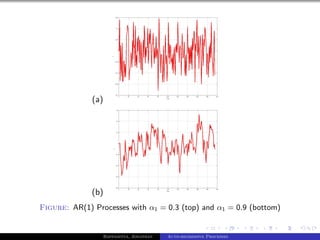
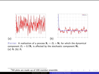
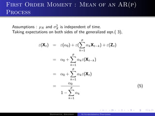
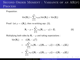
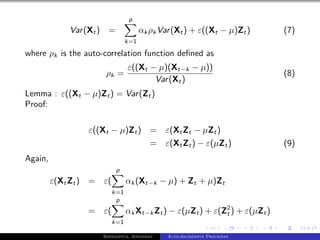
The document outlines auto-regressive (AR) processes of order p. It begins by introducing AR(p) processes formally and discussing white noise. It then derives the first and second moments of an AR(p) process. Specific details are provided about AR(1) and AR(2) processes, including equations for their variance as a function of the noise variance and AR coefficients. Examples of simulated AR(1) processes are shown for different coefficient values.

1. Auto-regressive Processes
B. Nag and J. Christophersen
MET - 6155
November 09, 2011

2. Outline of the talk
Introduction of AR(p) Processes
Formal Definition
White Noise
Deriving the First Moment
Deriving the Second Moment
Lag 1: AR(1)
Lag 2: AR(2)
Bappaditya, Jonathan Auto-regressive Processes

3. Introduction
Dynamics of many physical processes :
d 2 x(t) dx(t)
a2 2
+ a1 + a0 x(t) = z(t) (1)
dt dt
where z(t) is some external forcing function.
Time discretization yields
xt = α1 xt−1 + α2 xt−2 + zt (2)
Bappaditya, Jonathan Auto-regressive Processes

4. Formal Definition
Xt : t ∈ Z is an auto-regressive process of order p if there exist real
constants αk , k = 0, . . . , p, with αp = 0 and a white noise process
Zt : t ∈ Z such that
p
Xt = α0 + αk Xt−k + Zt (3)
k=1
Note : Xt is independent of the part of Zt that is in the future, but
depends on the parts of the noise processes that are in the present and
the past
Bappaditya, Jonathan Auto-regressive Processes

5. White Noise
Consider a time series :
Xt = Dt + Nt (4)
with Dt and Nt being the determined and stochastic (random)
components respectively.
If Dt is independent of Nt , then Dt is deterministic. Nt masks
deterministic oscillations when present.
Let us consider the case for k = 1.
Xt = α1 Xt−1 + Nt
= α1 (Dt−1 + Nt−1 ) + Nt
= α1 Dt−1 + α1 Nt−1 + Nt
where, α1 Nt−1 can be regarded as the contribution from the dynamics of
the white noise. The spectrum of a white noise process is flat and hence
the name.
Bappaditya, Jonathan Auto-regressive Processes

6. (a) (b)
Figure: A realization of a process Xt = Dt + Nt for which the dynamical
component Dt = 0.7Xt is affected by the stochastic component Nt .
(a) Nt (b) Xt
0 All plots are made up of 100 member ensemble
Bappaditya, Jonathan Auto-regressive Processes

7. First Order Moment : Mean of an AR(p)
Process
2
Assumptions : µX and σX is independent of time.
Taking expectations on both sides of the generalized eqn.( 3),
p
ε(Xt ) = ε(α0 ) + ε( αk Xt−k ) + ε(Zt )
k=1
p
= α0 + αk ε(Xt−k )
k=1
p
= α0 + αk ε(Xt )
k=1
α0
= p (5)
1− αk
k=1
Bappaditya, Jonathan Auto-regressive Processes

8. Second Order Moment : Variance of an AR(p)
Process
Proposition:
p
Var (Xt ) = αk ρk Var (Xt ) + Var (Zt )
k=1
Proof: Let µ = ε(Xt ), then re-writting eqn. (3),
p
Xt − µ = αk (Xt−k − µ) + Zt (6)
k=1
Multiplying both sides by Xt − µ and taking expectations :
Var (Xt ) = ε((Xt − µ)2 )
p
= ε( αk (Xt − µ)(Xt−k − µ)) + ε((Xt − µ)Zt )
k=1
p
= αk ε((Xt − µ)(Xt−k − µ)) + ε((Xt − µ)Zt )
k=1
Bappaditya, Jonathan Auto-regressive Processes

9. p
Var (Xt ) = αk ρk Var (Xt ) + ε((Xt − µ)Zt ) (7)
k=1
where ρk is the auto-correlation function defined as
ε((Xt − µ)(Xt−k − µ))
ρk = (8)
Var (Xt )
Lemma : ε((Xt − µ)Zt ) = Var (Zt )
Proof:
ε((Xt − µ)Zt ) = ε(Xt Zt − µZt )
= ε(Xt Zt ) − ε(µZt ) (9)
Again,
p
ε(Xt Zt ) = ε( αk (Xt−k − µ) + Zt + µ)Zt
k=1
p
= ε( αk Xt−k Zt ) − ε(µZt ) + ε(Z2 ) + ε(µZt )
t
k=1
Bappaditya, Jonathan Auto-regressive Processes

10. p
ε(Xt Zt ) = αk ε(Xt−k Zt ) + ε(Z2 )
t
k=1
p
= αk ε(Xt−k Zt ) + Var (Zt ) (10)
k=1
Since Xt is independent of the part of Zt that is in the future implies
Xt−k and Zt are independent. Hence
ε(Xt−k Zt ) = 0
Hence we get,
ε(Xt Zt ) = Var (Zt ) (11)
From equation (5),
ε(µZt ) = µε(Zt )
α0
= p ε(Zt )
1 − k=1 αk
α0
= p ×0
1 − k=1 αk
= 0
Bappaditya, Jonathan Auto-regressive Processes

11. Thus
ε((Xt − µ)Zt ) = Var (Zt ) (12)
and eqn. (7) reduces to
p
Var (Xt ) = αk ρk Var (Xt ) + Var (Zt )
k=1
Var (Zt )
Var (Xt ) = p (13)
1− αk ρk
k=1
Bappaditya, Jonathan Auto-regressive Processes

12. AR(1) Processes
Consider the following equation:
dx
a1 + a0 x = z(t) (14)
dt
Discretizing again :
a1 (x1 − xt−1 ) + a0 xt = zt
at xt − a1 xt−1 + a0 xt = zt
xt (a1 + a0 ) − a1 xt−1 = zt
Therefore we obtain :
xt = α1 xt−1 + zt (15)
a1 zt
where α1 = a1 +a0 and zt = a1 +a0
Bappaditya, Jonathan Auto-regressive Processes

13. AR(1) Processes Continued
Hence an AR(1) Process can be represented as
Xt = α1 Xt−1 + Zt (16)
For convinience we assume, α0 = 0 and ε(Xt ) = µ = 0
Expectation of the product of Xt with Xt−1 is
ε(Xt Xt−1 ) = α1 ε(X2 ) + ε(Zt Xt−1 )
t−1
Since Xt does not depend on the part of Zt that is in the future, hence
ε(Zt Xt−1 ) = 0
Also since the variance is independent of time,
ε(Xt Xt−1 ) = α1 ε(X2 )
t (17)
Hence,
ε(Xt Xt−1 )
α1 = (18)
Var (Xt )
Bappaditya, Jonathan Auto-regressive Processes

14. AR(1) Processes Continued
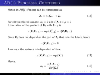
Substituting for k = 1, in eqn. (8), yields
ε(Xt Xt−1 )
ρ1 = (19)
Var (Xt )
Hence ρ1 = α1
Using this we can write eqn. (13) for an AR(1) process as
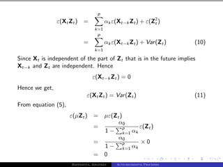
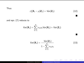
Var(Zt )
Var(Xt ) = p
1− k=1 αk ρk
2
σz
= 2 (20)
1 − α1
This result shows that the variance of the random variable Xt is a linear
2
function of the variance of the white noise σZ . This also shows that the
variance is also a nonlinear function of α1 .
If α1 ≈ 0, then the Var (Xt ) ≈ Var (Zt ). For α1 ∈ [0, 1], we see that
Var (Xt ) > Var (Zt ). As α1 approaches 1, the Var (Xt ) approaches ∞.
Bappaditya, Jonathan Auto-regressive Processes

15. (a)
(b)
Figure: AR(1) Processes with α1 = 0.3 (top) and α1 = 0.9 (bottom)
Bappaditya, Jonathan Auto-regressive Processes

16. AR(2) Processes
d 2 x(t) dx(t)
a2 + a1 + a0 x(t) = z(t) (21)
dt 2 dt
where z(t) is some external forcing function.
Time discretization yields
a2 (xt + xt−2 − 2xt−1 ) + a1 (xt − xt−1 ) + a0 xt = z(t)
(a0 + a1 + a2 )xt = (a1 + 2a2 )xt−1 − a2 xt−2 + zt
Alternatively,
xt = α1 xt−1 + α2 xt−2 + zt (22)
where
a1 + 2a2
α1 =
a0 + a1 + a2
a2
α2 = −
a0 + a1 + a2
1
zt = zt
a0 + a1 + a2
Bappaditya, Jonathan Auto-regressive Processes

17. and by = −0.8 (top)
Figure: AR(2) Processes with α1 = 0.9Generated α2CamScanner from intsig.com and with
α1 = α2 = 0.3 (bottom)
Bappaditya, Jonathan Auto-regressive Processes

18. Parameterizing AR(2) Processes
In order for AR(2) processes to be stationary, α1 and α2 must satisfy
three conditions:
(1) α1 + α2 < 1
(2) α1 − α2 < 1
(3) −1 < α2 < 1
This defines a triangular region for the (α1 , α2 )-plane.
Note that if α2 = 0 then we observe AR(1) processes where −1 < α1 < 1
defines the space for which α1 is stationary in an AR(1) model.
Bappaditya, Jonathan Auto-regressive Processes

19. Parameterizing AR(2) Processes Continued
Figure: Region of stationary points for AR(1) andbyAR(2) processes
Generated CamScanner from intsig.com
Bappaditya, Jonathan Auto-regressive Processes

20. Parameterizing AR(2) Processes Continued
The figure above shows:
AR(1) processes are special cases:
α1 > 0 shows exponential decay
α1 < 0 shows damped oscillations
α1 > 0 for most meteorological phenomena
The second parameter α2 :
More complex relationship between lags
For (0.9, −0.6), slow damped oscillation around 0
AR(2) models can represent pseudoperiodicity
Barometric pressure variations due to midlatitude synoptic systems
follow pseudoperiodic behavior
Bappaditya, Jonathan Auto-regressive Processes

21. Parameterizing AR(2) Processes Continued
(a) (b)
(c) (d)
Figure: Four synthetic time series illustrating some properties of
autoregressive models. (a) α1 = 0.0, α2 = 0.1, (b) α1 = 0.5, α2 = 0.1, (c)
α1 = 0.9, α2 = −0.6, (d) α1 = 0.09, α2 = 0.11
Bappaditya, Jonathan Auto-regressive Processes

22. References
von Storch, H., 1999: Statistical analysis in climate research, 1st ed.
Cambridge University, 494 pp.
Wilks, D., 1995: Statistical methods in the atmospheric sciences, 1st ed.
Academic Press, Inc., 467 pp.
Scheaffer, R., 1994: Introduction to probability and its applications,
2nd ed. Duxberry Press, 377 pp.
Bappaditya, Jonathan Auto-regressive Processes

23. Questions
??
Bappaditya, Jonathan Auto-regressive Processes