Downloaded 18 times

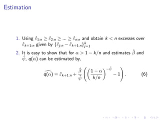
![Estimation
ˆ
First, m and h are estimated by m(Xt. ) and h(Xt. ) given the
ˆ
sample {(rt , Xt1 , · · · , Xtd )}n
t=1
rt −m(Xt. )
ˆ
Second, standardized residuals εt =
ˆ ˆ
h(Xt. )1/2
are used in
conjunction with extreme value theory to estimate q(α).
The exceedances of any random variable ( ) over a specified
nonstochastic threshhold u, i.e, Z = − u can be suitably
approximated by a generalized pareto distribution - GPD (with
location parameter equal to zero) given by,
−1/ψ
x
G (x; β, ψ) = 1 − 1 + ψ ,x ∈ D (5)
β
where D = [0, ∞) if ψ ≥ 0 and D = [0, −β/ψ] if ψ < 0.](https://image.slidesharecdn.com/fpday1pmmartins-filho-110621144009-phpapp01/85/Basic-concepts-and-how-to-measure-price-volatility-16-320.jpg)
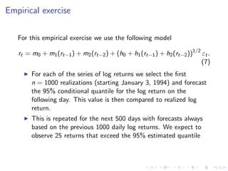
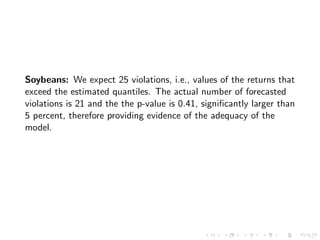
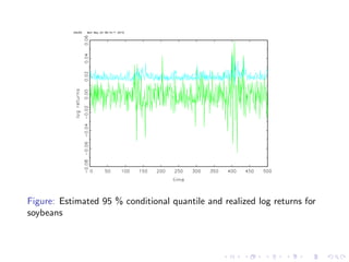
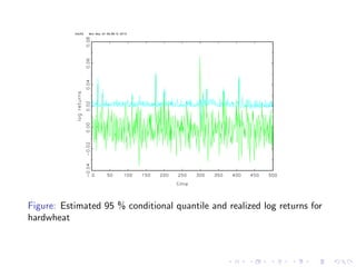

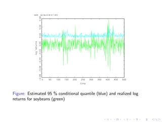
The document discusses the measurement of price volatility in agricultural commodities and the theoretical models used to understand it. It highlights the relationship between price volatility, expected profit losses, and resource allocation, while introducing statistical models like ARCH and GARCH for analyzing returns. An empirical exercise on log returns for soybeans and hard wheat is described, showing the effectiveness of the forecasting model used to estimate conditional quantiles.