Download as PDF, PPTX
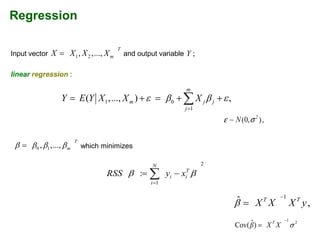
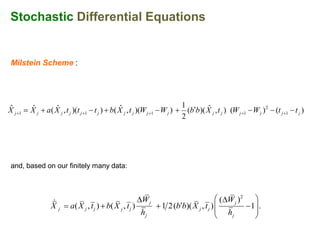
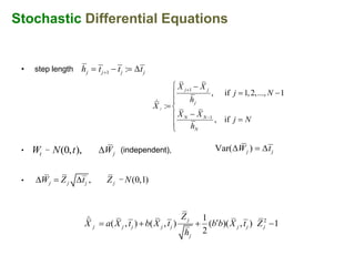
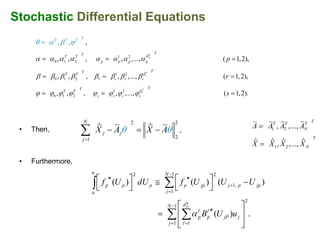
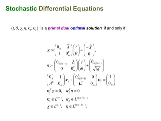
![Stochastic Differential Equations
dX t a( X t , t )dt b( X t , t )dWt
drift and diffusion term
Wt N (0, t ) (t [0, T ])
Wiener process](https://image.slidesharecdn.com/09-kiev2010-finance-sde-willi-100819074818-phpapp02/85/Parameter-Estimation-in-Stochastic-Differential-Equations-by-Continuous-Optimization-4-320.jpg)
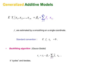
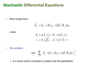
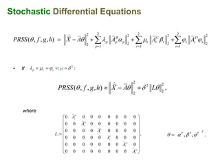
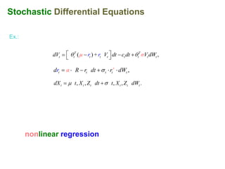
![Stochastic Differential Equations
dX t a( X t , t )dt b( X t , t )dWt
drift and diffusion term
Ex.: price, wealth, interest rate, volatility
processes
Wt N (0, t ) (t [0, T ])
Wiener process](https://image.slidesharecdn.com/09-kiev2010-finance-sde-willi-100819074818-phpapp02/85/Parameter-Estimation-in-Stochastic-Differential-Equations-by-Continuous-Optimization-5-320.jpg)
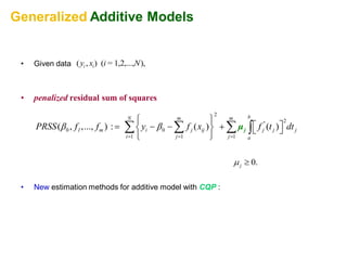
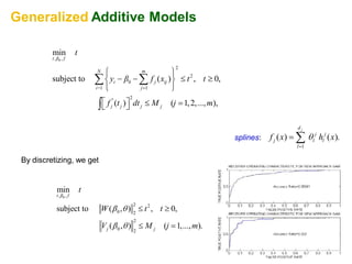
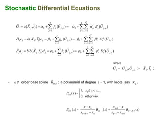
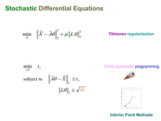
![MARS
y y
c-(x, )=[ (x )] c+(x, )=[ (x )] c-(x, )=[ (x )] c+(x,egressionx ith)]
r )=[ ( w
x x](https://image.slidesharecdn.com/09-kiev2010-finance-sde-willi-100819074818-phpapp02/85/Parameter-Estimation-in-Stochastic-Differential-Equations-by-Continuous-Optimization-11-320.jpg)
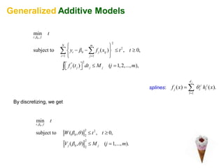
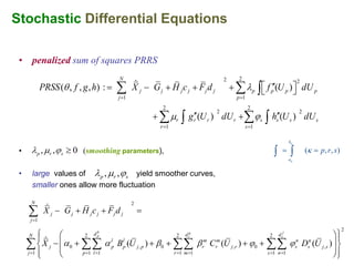
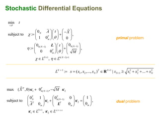
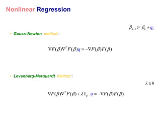
![Stochastic Differential Equations Revisited
dX t a( X t , t )dt b( X t , t )dWt
drift and diffusion term
Ex.: price, wealth, interest rate, volatility,
processes
Wt N (0, t ) (t [0, T ])
Wiener process](https://image.slidesharecdn.com/09-kiev2010-finance-sde-willi-100819074818-phpapp02/85/Parameter-Estimation-in-Stochastic-Differential-Equations-by-Continuous-Optimization-14-320.jpg)
![Stochastic Differential Equations Revisited
dX t a( X t , t )dt b( X t , t )dWt
drift and diffusion term
Ex.: bioinformatics, biotechnology
(fermentation, population dynamics)
Universiti Teknologi Malaysia
Wt N (0, t ) (t [0, T ])
Wiener process](https://image.slidesharecdn.com/09-kiev2010-finance-sde-willi-100819074818-phpapp02/85/Parameter-Estimation-in-Stochastic-Differential-Equations-by-Continuous-Optimization-15-320.jpg)
![Stochastic Differential Equations Revisited
dX t a( X t , t )dt b( X t , t )dWt
drift and diffusion term
Ex.: price, wealth, interest rate, volatility,
processes
Wt N (0, t ) (t [0, T ])
Wiener process](https://image.slidesharecdn.com/09-kiev2010-finance-sde-willi-100819074818-phpapp02/85/Parameter-Estimation-in-Stochastic-Differential-Equations-by-Continuous-Optimization-16-320.jpg)

The document discusses advancements in parameter estimation within stochastic differential equations and various statistical models. It covers topics such as nonlinear regression, conic quadratic programming, and portfolio optimization. The work highlights the balance between accuracy and stability in estimation methods, drawing from various mathematical principles and techniques.


![11.[104 111]analytical solution for telegraph equation by modified of sumudu ...](https://cdn.slidesharecdn.com/ss_thumbnails/11-104-111analyticalsolutionfortelegraphequationbymodifiedofsumudutransformelzakitransform-120513000219-phpapp01-thumbnail.jpg?width=640&height=640&fit=bounds)
![Lecture on nk [compatibility mode]](https://cdn.slidesharecdn.com/ss_thumbnails/lectureonnkcompatibilitymode-110825092241-phpapp01-thumbnail.jpg?width=640&height=640&fit=bounds)


