Panel slides

Panel Data Analysis October 2011
Introduction to Regression Models for Panel Data Analysis
Indiana University
Workshop in Methods
October 7, 2011
Professor Patricia A. McManus

WIM Panel Data Analysis October 2011| Page 1
What are Panel Data?
Panel data are a type of longitudinal data, or data collected at different
points in time. Three main types of longitudinal data:
 Time series data. Many observations (large t) on as few as one unit (small
N). Examples: stock price trends, aggregate national statistics.
 Pooled cross sections. Two or more independent samples of many units
(large N) drawn from the same population at different time periods:
o General Social Surveys
o US Decennial Census extracts
o Current Population Surveys*
 Panel data. Two or more observations (small t) on many units (large N).
o Panel surveys of households and individuals (PSID, NLSY, ANES)
o Data on organizations and firms at different time points
o Aggregated regional data over time
 This workshop is a basic introduction to the analysis of panel data. In
particular, I will cover the linear error components model.

Why Analyze Panel Data?
 We are interested in describing change over time
o social change, e.g. changing attitudes, behaviors, social relationships
o individual growth or development, e.g. life-course studies, child
development, career trajectories, school achievement
o occurrence (or non-occurrence) of events
 We want superior estimates trends in social phenomena
o Panel models can be used to inform policy – e.g. health, obesity
o Multiple observations on each unit can provide superior estimates as
compared to cross-sectional models of association
 We want to estimate causal models
o Policy evaluation
o Estimation of treatment effects

What kind of data are required for panel analysis?
 Basic panel methods require at least two “waves” of measurement.
Consider student GPAs and job hours during two semesters of college.
 One way to organize the panel data is to create a single record for each
combination of unit and time period:
StudentID Semester Female HSGPA GPA JobHrs
17 5 0 2.8 3.0 0
17 6 0 2.8 2.1 20
23 5 1 2.5 2.2 10
23 6 1 2.5 2.5 10
 Notice that the data include:
o A time-invariant unique identifier for each unit (StudentID)
o A time-varying outcome (GPA)
o An indicator for time (Semester).
 Panel datasets can include other time-varying or time-invariant variables

 An alternative way to structure the data is to keep all the measures
related to each student in a single record. This is sometimes called
“wide” format.
StudentID Female HSGPA GPA5 JobHrs5 GPA6 JobHrs6
17 0 2.8 3.0 0 2.1 20
23 1 2.5 2.2 10 2.5 10
o Why are there two variables for GPA and JobHrs ?
o Why is there only one variable for gender and high school GPA?
o Where is the indicator for time?

Estimation Techniques for Panel Models
We can write a simple panel equation predicting GPA from hours worked:
0
it it T it H it J it
GPA TERM HSGPA JOB v
 General Linear Model is the foundation of linear panel model estimation
o Ordinary Least Squares (OLS)
o Weighted least squares (WLS)
o Generalized least squares (GLS)
Least-squares estimation of panel models typically entails three steps:
(a) Data transformation or first-stage estimation
(b) Estimation of the parameters using Ordinary Least Squares
(c) Estimation of the variance-covariance matrix of the estimates (VCE)
Parameter estimates are sometimes refined using iteratively reweighted
least squares (IRLS), a maximum likelihood estimator.

Basic Questions for the Panel Analyst
What’s the story you want to tell?
 Is this a descriptive analysis? Less worry, fewer controls are usually better.
 Is this an attempt at causal analysis using observational data? Careful
specification AND theory is essential.
How does time matter?
 Some analyses, e.g. difference-in-difference analysis associates time with
an event (before and after)
 Some analyses may be interested in growth trajectories.
 Panel analysis may be appropriate even if time is irrelevant. Panel models
using cross-sectional data collected at fixed periods of time generally use
dummy variables for each time period in a two-way specification with
fixed-effects for time.
Are the data up to the demands of the analysis?
 Panel analysis is data-intensive. Are two waves enough?
 Can you perform the necessary specification tests?
 How will you address panel attrition?

Review of the Classical Linear Regression Model
0 1 1 2 2 ...
i i i ki k i
y x x x u , i=1,2,3,…N
Where we assume that the linear model is correct and:
 Covariates are Exogenous: 1 2
| , ,.., 0
i i i ki
E u x x x
 Uncorrelated errors: , 0
i j
Cov u u
 Homoskedastic errors: 2
1 2
| , ,...,
i i i i ki
Var u Var y x x x
If assumptions do not hold, OLS estimates are BIASED and/or INEFFICIENT
 Biased - Expected value of parameter estimate is different from true.
o Consistency. If an estimator is unbiased, or if the bias shrinks as the
sample size increases, we say it is CONSISTENT
 Inefficient - (Informally) Estimator is less accurate as sample size
increases than an alternative estimator.
o Estimators that take full advantage of information more efficient

OLS Bias Due to Endogeneity
 Omitted Variable Bias
o Intervening variables, selectivity
 Measurement Error in the Covariates
 Simultaneity Bias
o Feedback loops
o Omitted variables
Conventional regression-based strategies to address endogeneity bias
 Instrumental Variables estimation
 Structural Equations Models
 Propensity score estimation
 Fixed effects panel models

OLS Inefficiency due to Correlated Errors
Many data structures are susceptible to error correlation:
 Hierarchical data sample multiple individuals from each unit, e.g.
household members, employees in firms, multiple pupils from each school.
 Multistage probability samples often incorporate cluster-based sampling
designs with errors that may be correlated within clusters.
 Repeated observations data often show within-unit error correlation.
 Time series data often have errors that are serially correlated, that is,
correlated over time.
 Panel data have errors that can be correlated within unit (e.g. individuals),
within period.
Conventional regression-based strategies to address correlated errors
 Cluster-consistent covariance matrix estimator to adjust standard errors.
 Generalized Least Squares instead of OLS to exploit correlation structure.

Linear Panel Data Model (LPM)
Suppose the data are on each cross-section unit over T time periods:
, 1 , 1 1 , 1
, 2 , 2 2 , 1
, , ,
'
'
:::
'
i t i t t i t
i t i t t i t
i T i T T i T
y u
y u
y u
x
x
x
, t=1,2,…,T
We can express this concisely using i
y to represent the vector of individual
outcomes for person i across all time periods:
i i i
y X u , where '
, 1 , 2
, ,...,
i i t i t iT
y y y
y
For comparison, begin with two conventional OLS linear regression models,
one for each period. Note that the variables female highgpa (HS
GPA) is time-invariant.

OLS Results for each term:
Term 5 GPA Term 6 GPA
Estimate SE t-stat Estimate SE t-stat
Intercept 3.02 0.17 17.8 3.02 0.17 18.3
jobhrs -0.182 0.05 -4.0 -0.174 0.05 -3.6
female 0.108 0.04 2.5 0.145 0.05 3.2
highgpa -0.004 0.04 -0.1 0.003 0.04 0.1
Pooled OLS Results for both terms:
Term 5&6 GPA Term 5&6 GPA (Clustered SE)
Estimate SE t-stat Estimate SE t-stat
Intercept 2.97 0.17 25.1 2.97 0.17 17.2
jobhrs -0.178 0.05 -5.4 -0.178 0.05 -5.8
female 0.125 0.04 4.1 0.125 0.04 3.0
highgpa -0.0001 0.03 -0.01 0.0001 0.03 -0.0004
term6 0.095 0.016 6.1 0.095 0.016 6.1

Linear Unobserved Effects Panel Data Model
 Motivation: Unobserved heterogeneity
Suppose we have a model with an unobserved, time-constant variable c:
0 1 1 2 2 ... k k
y x x x c u
Where u is uncorrelated with all explanatory variables in x.
Because c is unobserved it is absorbed into the error term, so
we can write the model as follows:
0 1 1 2 2 ... k k
y x x x v
v c u
The error term v consists of two components, an “idiosyncratic”
component u and an “unobserved heterogeneity” component c .

OLS Estimation of the Error Components Model
 If the unobserved heterogeneity i
c is correlated with one or more of the
explanatory variables, OLS parameter estimates are biased and
inconsistent.
 If the unobserved heterogeneity c is uncorrelated with the explanatory
variables in i
x , OLS is unbiased even in a single cross-section.
 If we have more than one observation on any unit, the errors will be
correlated and OLS estimates will be inefficient
1 1 1
2 2 2
,1 0 1 1 2 2 ,1
,2 0 1 1 2 2 ,2
,1 ,1
,2 ,2
,1 ,2
...
...
, ) 0
i i i
i i i
i k k i
i k k i
i i i
i i i
i i
y x x x v
y x x x v
v c u
v c u
cov(v v

 Unobserved Heterogeneity in Panel Data
Suppose the data are on each cross-section unit over T time periods.
This is an unobserved effects model (UEM), also called the error
components model. We can write the model for each time period:
1 1
2 2
i i i i
i i i i
iT iT i iT
y c u
y c u
y c u
1
2
x
x
x
,
Where there are T observations on outcome y for person i,
it
x is a vector of explanatory variables measured at time t,
i
c is unobserved in all periods but constant over time
it
u is a time-varying idiosyncratic error
Define it i it
v c u as the composite error.

Consistent estimation of the Error Components Model with Pooled OLS
If we assume no contemporaneous correlation of the errors and the
explanatory variables, pooled OLS estimation is consistent:
'
( )
it it
E u
x 0 and '
( )
it i
E c
x 0, t=1,2,…,T
Efficient estimation of the Error Components Model with Pooled OLS
Even if estimation is consistent, pooled OLS may not be efficient.
 One strategy is to combine pooled OLS with cluster-consistent standard
errors.
 Panel GLS methods may be preferred.
In the next sections, we consider the dominant approaches to estimation
of the error components panel model: fixed effects and random effects.

Illustration of Within-unit correlation. Peak-flow Measurements
200
300
400
500
600
700
1 2 3 4 5 6 7 8 9 10 11 12 13 14 15 16 17
Subject ID
Wright Peak #1 Wright Peak #2

Just a few panel data examples:
Propper and Van Reenen (2010)
Effect of regulation of nursing pay on hospital quality
Data: 209 NHS Hospitals in the UK 1997-2005
Western, Bruce (2002)
Effect of Incarceration on wages and income inequality
Data: NLSY
Cherlin, Chase-Lansdale and McRae (1998)
Effect of parental divorce on mental health over life-course
Data: British Cohort Study
Jacobs and Carmichael (2002)
Determinants of Death Penalty in US states
Data: US Census 1970, 1980, 1990 + other sources
Baum and Lake (2003)
Effect of Democracy on Human Capital and Economic Growth
Data: Aggregate data on 128 countries over 30 years

Fixed Effects Methods for Panel Data
Suppose the unobserved effect i
c is correlated with the covariates.
Example: Motherhood wage penalty
 We observe that mothers earn less than other women, cet par.
ˆ 0.08
OLS
KIDS in a log wage model suggests that each additional
child reduces mothers’ hourly wages by about 8%
But if women who are less oriented towards work are also more likely to
have more children, omitting “work orientations” from the model will bias
the coefficient on children.
 Fixed-effects methods transform the model to remove i
c
ˆ 0.03
FE
KIDS FE estimates a persistent but much smaller penalty.

 Caution: Fixed effects has some disadvantages
 FE is not a panacea for all sources of endogeneity bias.
time-varying unobserved effects
time-varying measurement error
simultaneity or feedback loops
 All time-constant effects are removed.
No estimation of effects of race, gender, birth order, etc.
Poor estimates if little variation (e.g. education in adulthood)
 FE trades consistency for efficiency.
FE uses only within-unit change, ignores between-unit variation.
Parameter estimates may be imprecise, standard errors large.
 Despite limitations, FE is an indispensable tool in the panel analyst’s
toolbox.
Fixed Effects Transformation - the “Within” Estimator

Suppose we have the UEM model:
'
it it i it
y c u
x , t=1,2,…,T
For each unit, average this equation over all time periods t:
'
i i i i
y c u
x
Subtract the within-unit average from each observation on that unit:
' '
it i it i i i it i
y y c c u u
x x , t=1,2,…,T
This is the fixed effects transformation. We can write it as:
'
it it it
y u
x ,
where 0
i i
c c and it it i
y y y , it it i
x x x , it it i
u u u
and it
x does not contain an intercept term.

The fixed-effects estimator, also called the within estimator, applies pooled
OLS to the transformed equation:
1 1
' ' ' '
1 1 1 1 1 1
ˆ
N N N T N T
FE i i i i it it it it
i i i t i t
y
X X X y x x x
Recall the student GPA Data:
17 5 0 2.8 3.0 0
17 6 0 2.8 2.1 20
23 5 1 2.5 2.2 10
23 6 1 2.5 2.5 10
After applying the fixed-effects transform, the demeaned (mean-centered)
data:
StudentID Semester CFemale CHSGPA CGPA CJobHrs
17 -.5 0 0 .45 -10
17 .5 0 0 -.45 10
23 -.5 0 0 -.15 0
23 .5 0 0 .15 0

Fixed Effects Dummy Variables Regression
Up to now, we’ve treated the unobservables i
c as random variables:
'
it it i it
y c u
x
An alternative approach is to treat i
c as a fixed parameter for each unit. In
this case, we can use dummy variables regression to estimate i
c .
Step one: Create a dummy variable for each of sample unit i
Step two: Substitute the vector of N-1 dummies for i
c :
'
1 2 3
2 3 ...
it it N it
y d d dN u
x ,
(where the intercept 1 estimates the effect when 1
d =1)
Step three: Estimate the equation using pooled OLS.
 The fixed effects dummy variables (FEDV) estimator produces precisely
the same coefficient vector and standard errors as the FE estimator.

*** Practical asides
One way or two? Sometimes you will see “one-way” or “two-way” FE.
One-way fixed effects error components model - only the unit effects are
conditioned out.
Two-way fixed effects error components model – both the unit effects and
period effects are conditioned out.
In the conventional FE model with large N and small T, it is a simple
matter to create dummy variables for each period, and most panel models
will include controls for period effects.
Statistical Software
Most statistical packages offer several alternatives for estimating the FEM.
STATA xtreg areg reg (with factor variables)
SAS proc panel proc glm (with “absorb” statement)

First Differencing Methods
 The first difference (FD) model transforms the UEM model to remove the
unobserved effects i
c
 FD is sometimes called a first-difference fixed effects model
Suppose we have the unobserved effects model (UEM):
'
it it i it
y c u
x ,
For each observation, subtract the previous within-unit observation:
' '
, 1 , 1 , 1
it i t it i t i i it i t
y y c c u u
x x
This is the first-difference transformation. We can write it as:
'
it it it
y u
x ,
where 0
i
c and it
x does not contain an intercept term.

Consider the two-period data student GPA Data:
17 5 0 2.8 3.0 0
17 6 0 2.8 2.1 20
23 5 1 2.5 2.2 10
23 6 1 2.5 2.5 10
After applying the first-difference transform, the differenced data:
StudentID DSemester dFemale dHSGPA dGPA dJobHrs
17 . . . . .
17 1 0 0 -.9 20
23 . . . . .
23 1 0 0 .3 0

Fixed Effects and First Differences in the Two-Period Case
FE (Within) Transform
StudentID Semester CFemale CHSGPA CGPA CJobHrs
17 -.5 0 0 .45 -10
17 .5 0 0 -.45 10
23 -.5 0 0 -.15 0
23 .5 0 0 .15 0
FD (Differenced) Transform:
StudentID DSemester dFemale dHSGPA dGPA dJobHrs
17 1 0 0 -.9 20
23 1 0 0 .3 0
Compare the transformed (FE) and differenced (FD) data. Each FD variable
is equal to the difference between the second-period FE demeaned
variable and the first-period demeaned variable.
This symmetry will always be present in the two-period panel model.
As a result, the parameter estimates for the two-period panel model can
be obtained using FD or FE, with identical results. Not so if T>2 !

FE and FD Results for two terms:
Term 5&6 GPA (FE, N=400) Term 5&6 GPA (FD, N=200)
Estimate SE Estimate SE________
jobhrs -0.0640159 0.0223835 -0.0640159 0.0223835
term6 0.1133996 0.0125627 0.1133996 0.0125627
FE and FD Results for six terms:
Terms 1-6 GPA (FE, N=1200) Term 1-6 GPA (FD, N=1000)
Estimate SE Estimate SE________
jobhrs -0.1285521 0.0188415 -0.087316 0.0174187
term 0.1037983 0.0040011 0.1066726 0.0091661

Difference-in-Difference Model for Panel Data using FD
Suppose we have a treatment that affects some but not all units in the
population. The “difference-in-differences” estimator is the difference
between the change over time in the treatment group and the change over
time in the control:
,2 ,1 ,2 ,1
B B A A
DID y y y y
If we have panel data from a time period prior to treatment and a second
observation drawn after the treatment event, we can study treatment
effects using 2-period panel data FD and DID:
1 0 1 1 1
2 0 1 2 2
i PD i TREAT i i
i PD i TREAT i i
y PERIOD treatment v
y PERIOD treatment v
, and
Where 1
i
treatment indicates treatment, zero for all at time t=1
PERIOD is a dummy for the time period.

The first difference model for difference-in-difference:
i PD TREAT i i
y treatment v
Where the intercept is replaced by a period effect ( 1
PERIOD for all
units and the change in treatment is either 0 or 1.
Designate A as the control group (i.e. 0
i A
treatment )
Designate B as the treatment group (i.e. 1
i B
treatment )
i PD TREAT i i
y treatment v
Difference in differences estimator:
,2 ,1 ,2 ,1
ˆ ˆ ˆ ˆ
) (
ˆ
B B A A
PD TREAT i B PD TREAT i A
TREAT
DID y y y y
treatment treatment
e.g. Card & Krueger (2000) Minimum Wage increases & Employment

Choosing an Estimator: Fixed Effects vs. First Differences (FE vs FD)
 If T=2, (two period model) the FE and FD are identical
 If T>2 FE is more efficient than if there is no serial correlation of the
idiosyncratic errors.
 If T>2 FD is more efficient if there is serial correlation.
 If the unobserved error is not correlated with the covariates, neither the
FE nor the FD model is efficient.

Why not Just Use a Lagged Dependent Variable?
Source: David Johnson. Journal of Marriage and Family, Vol. 67, No. 4 (Nov., 2005), pp. 1061-1075

Random Effects Methods
If we can assume that the unobserved heterogeneity will not bias the
estimates:
 Fixed effects methods are inefficient. They throw away information.
 Pooled OLS is inefficient because it does not exploit the autocorrelation
in the composite error term.
 Random effects methods use feasible GLS estimation (RE FGLS) to
exploit within-cluster correlation
 Random effects estimation is more efficient than FE or OLS
 The “random effects assumption” of no bias due to i
c is more stringent
1
( | ,..., ) ( ) 0
i i iT i
E c E c
x x

A Conventional FGLS Random Effects Estimator
Assume the errors are correlated within each unit
Assume the errors are uncorrelated across units
Assume the variance in the composite errors is equal to the sum of the
variances in the unobserved effect i
c and the idiosyncratic error i
u :
2 2 2
v u c
RE strategy: If 2 2 2
v u c , find estimators such that 2 2 2
ˆ ˆ ˆ
v u c

Practical Feature of Random Effects Estimation
 Recall that the fixed effects “within” estimator essentially transforms
the data by centering each variable on the unit-specific mean.
OLS is then performed on the “fully demeaned” transformed data.
 The random effects estimator essentially transforms the data by
“partially demeaning” each variable. Instead of subtracting the entire
unit-specific mean, only part of the mean is subtracted.
The demeaning factor is between 0 and 1, with the specific value
based on the variance components estimation.
 Random effects routines are standard in statistical software packages:
SAS: PROC GLM or PROC PANEL
STATA: xtreg

RE Results compared to pooled OLS Results for two terms:
RE Term 5&6 GPA OLS Term 5&6 GPA
Estimate SE z-stat Estimate SE t-stat
Intercept 2.81 0.16 18.0 2.97 0.17 17.2
jobhrs -0.108 0.02 -4.8 -0.178 0.05 -5.8
female 0.126 0.04 3.0 0.125 0.04 3.0
highgpa -0.001 0.03 -0.04 0.0001 0.03 -0.0004
term6 0.096 0.015 5.6 0.095 0.016 6.1
RE Results for six terms:
Terms 1-6 GPA (FE, N=400)
Estimate SE
Intercept 2.41 0.10 23.5
jobhrs -0.129 0.02 -7.0
female 0.086 0.03 2.8
highgpa -0.030 0.02 1.2
term 0.088 0.006 13.6

Random Effects or Fixed Effects - How to decide?
Hausman test for the Exogeneity of the Unobserved Error Component
If the unobserved effects are exogenous, the FE and RE are asymptotically
equivalent. This suggests the null hypothesis for the Hausman test:
0
ˆ ˆ
: RE FE
H ,
where ˆ
RE and ˆ
FE are coefficient vectors for the time-varying explanatory
variables, excluding the time variables.
If the null hypothesis is rejected, we conclude that RE is inconsistent, and the
FE model is preferred.
If the null hypothesis cannot be rejected, random effects is preferred because
it is a more efficient estimator.

Hausman Test in Stata:
. xtreg gpa job sex highgpa,fe
. estimates store fe
. xtreg gpa job sex highgpa,re
. estimates store re
. hausman fe re
---- Coefficients ----
| (b) (B) (b-B) sqrt(diag(V_b-V_B))
| fe re Difference S.E.
-------------+---------------------------------------------------------------
job | -.0748115 -.1232374 .048426 .0088051
-----------------------------------------------------------------------------
b = consistent under Ho and Ha; obtained from xtreg
B = inconsistent under Ha, efficient under Ho; obtained from xtreg
Test: Ho: difference in coefficients not systematic
chi2(1) = (b-B)'[(V_b-V_B)^(-1)](b-B)
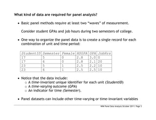
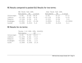
= 30.25
Prob>chi2 = 0.0000
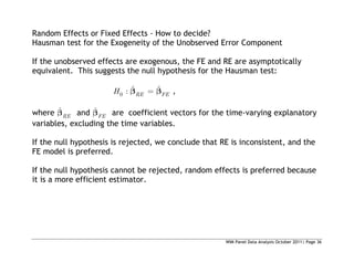
 We reject the null and conclude the fixed effects estimator is appropriate.

Interpretation of Results from the Error Components Model
Since the UEM model is derived as a levels model, coefficients can be
interpreted much the same as interpretations of a conventional OLS
model, but there are nuances:
For example, suppose we estimate the relationship between marriage and
men’s wages, ˆ 0.05
MARRIED in every model.
 Pooled OLS cross-section coefficients contain information about average
differences between units.
[ | ]
it it it i
E y c
x x
This is a population-averaged effect. On average, married men earn 5%
more than men who are not married.
This says nothing about the causal effect of marriage on men’s earnings.

 RE/FE/FD estimate average effects within units.
If the unobserved effects are exogenous these are asymptotically
equivalent to the population averaged effect.
[ | , ]
it it i it
E y c
x x
This is sometimes called an average treatment effect. On average,
entering marriage increases men’s earnings by 5%.
 RE coefficients represent average change within units, estimated from all
units whether they experience change or not.
 FE and FD coefficients represent average changes within units, only for
units that did experience change
This is akin to a treatment effect among the treated. On average, men
who married increased their earnings by 5%.

Best Practices
Theorize the model
 What exactly does this unobserved heterogeneity represent?
 Why would you expect it to be correlated / uncorrelated with the
regressors?
Specification Testing for Panel Analysis - Interval/Continuous Outcomes
 Before ruling out pooled OLS, test for appropriateness of panel methods
vs. pooled ordinary least square.
 Optional: Obtain intraclass correlation coefficient (ICC) as indicator of the
extent of within-unit clustering. This is a descriptive statistic, not a test.
 Specification tests for strict exogeneity
 Test for serial correlation in the idiosyncratic errors
 Hausman test for random effects vs. fixed effects

Extensions
FE Models with Time-Invariant Predictors
 Interactions between time and covariate
Panel Models for Categorical Outcomes
 Fixed effects logit and random effects logit for binary outcomes
 Fixed and random effects Poisson models can be used for count outcomes.
 Population averaged models can be estimated using General Estimation
Equations (GEE).
Dynamic panel models i.e. lagged dependent variable as a covariate:
0 , 1
it i t GPA it T it H it J it
GPA GPA TERM HSGPA JOB v
 GLM models for instrumental variables (IV) estimation
 Generalized Method of Moments (GMM) is used for some dynamic panel
models because it allows a flexible specification of the instruments

Panel slides

Recommended

Recommended

More Related Content

What's hot

What's hot (20)

Similar to Panel slides

Similar to Panel slides (20)

Recently uploaded

Recently uploaded (20)

Panel slides