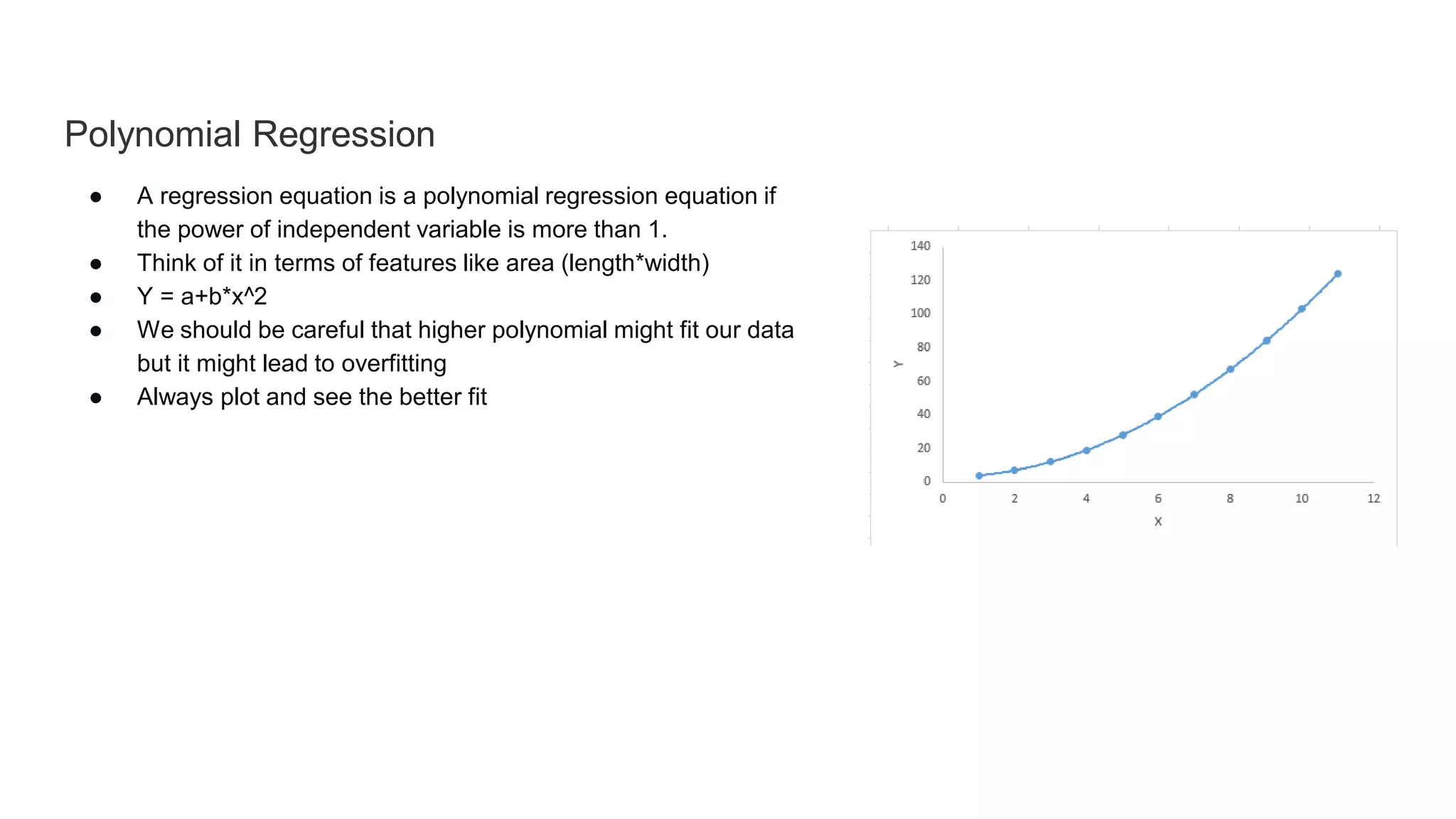
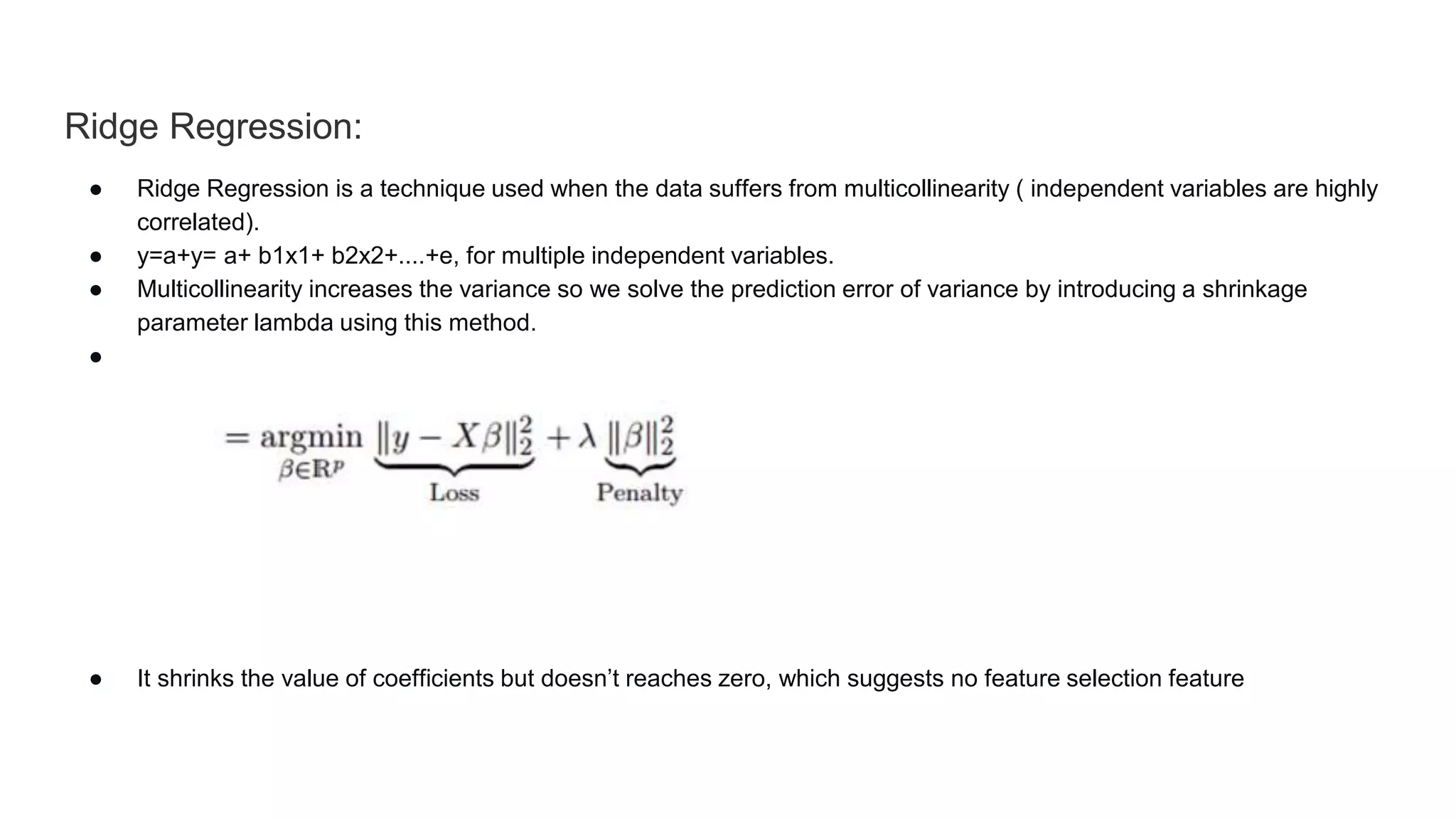
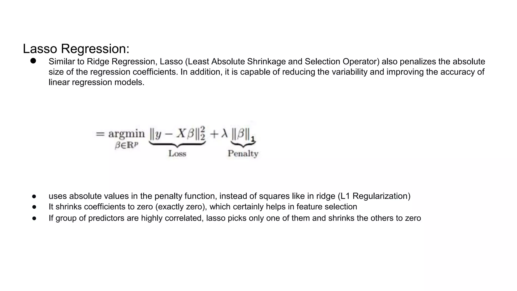
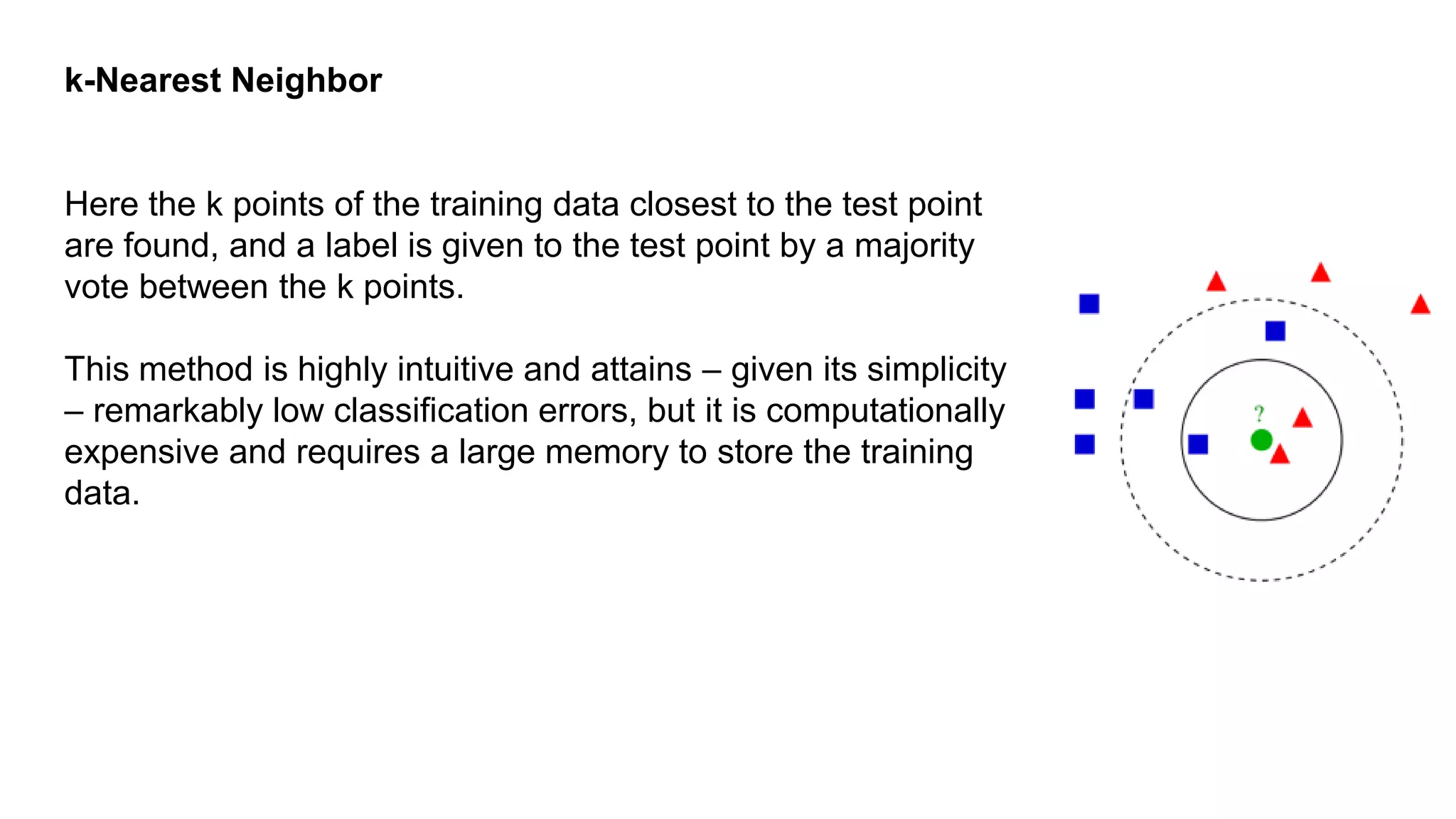
- Linear regression estimates the relationship between continuous dependent and independent variables using a best fit line. Multiple linear regression uses multiple independent variables while simple linear regression uses one. - Logistic regression applies a sigmoid function to linear regression when the dependent variable is binary. It handles non-linear relationships between variables. - Polynomial regression uses higher powers of independent variables which may lead to overfitting so model fit must be checked. - Stepwise regression automatically selects independent variables using forward selection or backward elimination. Ridge and lasso regression address multicollinearity through regularization. Elastic net is a hybrid of ridge and lasso. - Classification algorithms include k-nearest neighbors, decision trees, support vector machines, and naive Bayes which use probability

1. Supervising
Supervised Algorithms
-Prudhvi

3. Regression Algorithms(regression analysis estimates the relationship between two or more variables. )

4. Bias and Variance

5. Linear Regression:
● In this technique, the dependent variable is continuous, independent
variables can be continuous or discrete, and nature of regression line is
linear.
● Linear Regression establishes a relationship between dependent variable
(Y) and one or more independent variables (X) using a best fit straight
line (also known as regression line).
● Equation ( Y = W*X+b) [Y=dependent X=independent, b = bias]
● The difference between simple linear regression and multiple linear
regression is that, multiple linear regression has (>1) independent variables,
whereas simple linear regression has only 1 independent variable.
● We obtain the best fit by least squares method

6. Logistic Regression:
● We should use logistic regression when the dependent variable is
binary (0/ 1, True/ False, Yes/ No) in nature. Here the value of Y
ranges from 0 to 1 and it can represented by following equation.
● Simply it can be defined as applying sigmoid function to linear
regression.
● Y = sigmoid(A.X+b)
● Logistic regression doesn’t require linear relationship between
dependent and independent variables. It can handle various types of
relationships because it applies a non-linear log transformation to the
predicted odds ratio
● The independent variables should not be correlated with each other
i.e. no multi collinearity.

7. Polynomial Regression
● A regression equation is a polynomial regression equation if
the power of independent variable is more than 1.
● Think of it in terms of features like area (length*width)
● Y = a+b*x^2
● We should be careful that higher polynomial might fit our data
but it might lead to overfitting
● Always plot and see the better fit

8. Stepwise Regression
● This is considered when we deal with multiple independent variables.
● In this technique, the selection of independent variables is done with the help of an automatic process, which
involves no human intervention.
● Stepwise regression basically fits the regression model by adding/dropping covariates one at a time based on a
specified criterion.
● Standard stepwise regression does two things. It adds and removes predictors as needed for each step.
● Forward selection starts with most significant predictor in the model and adds variable for each step.
● Backward elimination starts with all predictors in the model and removes the least significant variable for each step.
● Good while handling higher dimensionality datasets

9. Ridge Regression:
● Ridge Regression is a technique used when the data suffers from multicollinearity ( independent variables are highly
correlated).
● y=a+y= a+ b1x1+ b2x2+....+e, for multiple independent variables.
● Multicollinearity increases the variance so we solve the prediction error of variance by introducing a shrinkage
parameter lambda using this method.
● L2 regularization is used
● It shrinks the value of coefficients but doesn’t reaches zero, which suggests no feature selection feature

10. Lasso Regression:
● Similar to Ridge Regression, Lasso (Least Absolute Shrinkage and Selection Operator) also penalizes the absolute
size of the regression coefficients. In addition, it is capable of reducing the variability and improving the accuracy of
linear regression models.
● uses absolute values in the penalty function, instead of squares like in ridge (L1 Regularization)
● It shrinks coefficients to zero (exactly zero), which certainly helps in feature selection
● If group of predictors are highly correlated, lasso picks only one of them and shrinks the others to zero

11. ElasticNet Regression:
● ElasticNet is hybrid of Lasso and Ridge Regression techniques. It is trained with L1 and L2 prior as regularizer.
Elastic-net is useful when there are multiple features which are correlated. Lasso is likely to pick one of these at
random, while elastic-net is likely to pick both
● It encourages group effect in case of highly correlated variables
● There are no limitations on the number of selected variables
● It can suffer with double shrinkage

12. Classification
classification task is to find a functional mapping between the input data X, describing the input pattern, to a class label Y
(e.g. −1 or +1), such that Y = f(X).

13. k-Nearest Neighbor
Here the k points of the training data closest to the test point
are found, and a label is given to the test point by a majority
vote between the k points.
This method is highly intuitive and attains – given its simplicity
– remarkably low classification errors, but it is computationally
expensive and requires a large memory to store the training
data.

14. Decision Trees
● Another intuitive class of classification algorithms are
decision trees. These algorithms solve the classification
problem by repeatedly partitioning the input space, so as to
build a tree whose nodes are as pure as possible (that is,
they contain
points of a single class).
● Classification of a new test point is achieved by moving
from top to bottom along the branches of the tree, start-
ing from the root node, until a terminal node is reached.
● Decision trees are simple yet effective classification
schemes for small datasets.
● The computational complexity scales unfavorably with the
number of dimensions of the data. Large datasets tend to
result in complicated trees, which in turn require a large
memory for storage.

15. Support Vector Machines
They work by mapping the training data into a feature space by the aid of a so-called kernel
function and then separating the data using a large margin hyperplane.
Intuitively, the kernel computes a similarity between two given examples. Most commonly used
kernel functions are RBF kernels ′ and polynomial kernels.
The SVM finds a large margin separation between the training examples and previously unseen
examples will often be close to the training examples.
Hence, the large margin then ensures that these examples are correctly classified as well, i.e., the
decision rule generalizes.
SVMs have an interpretation as a hyperplane separation in a high dimensional feature space.
Support Vector Machines have been used on million dimensional data sets.

16. Naive Bayes:
Naive Bayes classifiers are a family of simple probabilistic classifiers based on
applying Bayes’ theorem with strong (naive) independence assumptions between
the features.
with P(A|B) is posterior probability, P(B|A) is likelihood, P(A) is class prior probability,
and P(B) is predictor prior probability.
Useful when we we have high dimensions

20. Just for fun

21. Thank you :)