Linear Regression
PREPARED BY:PROF. SHAKUNTLA RAVANI
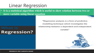
• It is a statistical algorithm which is useful to show relation between two or
more variable using linear equation
5.
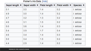
Linear Regression
PREPARED BY:PROF. SHAKUNTLA RAVANI
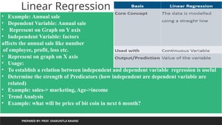
• Example: Annual sale
• Dependent Variable: Annual sale
• Represent on Graph on Y axis
• Independent Variable: factors
affects the annual sale like number
of employee, profit, loss etc.
• Represent on graph on X axis
• Usage:
• To establish a relation between independent and dependent variable regression is useful
• Determine the strength of Predicators (how independent are dependent variable are
related)
• Example: sales-> marketing, Age->income
• Trend Analysis
• Example: what will be price of bit coin in next 6 month?
6.
Linear Regression
PREPARED BY:PROF. SHAKUNTLA RAVANI
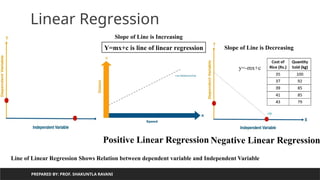
Positive Linear Regression Negative Linear Regression
Slope of Line is Increasing
Slope of Line is Decreasing
Y=mx+c is line of linear regression
Line of Linear Regression Shows Relation between dependent variable and Independent Variable
y=-mx+c
7.
PREPARED BY: PROF.SHAKUNTLA RAVANI
Linear Regression
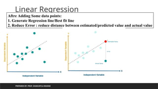
Aftre Adding Some data points:
1. Generate Regression line/Best fit line
2. Reduce Error : reduce distance between estimated/predicted value and actual value
8.
PREPARED BY: PROF.SHAKUNTLA RAVANI
Linear Regression
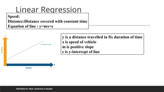
Speed:
Distance:Distance covered with constant time
Equation of line : y=mx+c
y is a distance travelled in fix duration of time
x is speed of vehicle
m is positive slope
c is y-intercept of line
9.
PREPARED BY: PROF.SHAKUNTLA RAVANI
Types of Linear regression
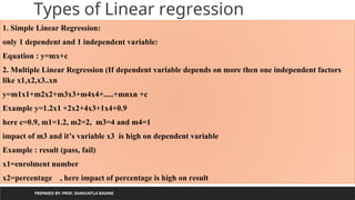
1. Simple Linear Regression:
only 1 dependent and 1 independent variable:
Equation : y=mx+c
2. Multiple Linear Regression (If dependent variable depends on more then one independent factors
like x1,x2,x3..xn
y=m1x1+m2x2+m3x3+m4x4+.....+mnxn +c
Example y=1.2x1 +2x2+4x3+1x4+0.9
here c=0.9, m1=1.2, m2=2, m3=4 and m4=1
impact of m3 and it’s variable x3 is high on dependent variable
Example : result (pass, fail)
x1=enrolment number
x2=percentage , here impact of percentage is high on result
10.
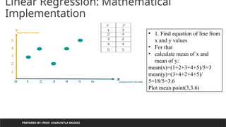
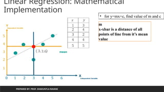
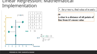
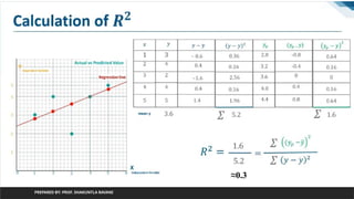
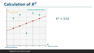
Linear Regression: Mathematical
Implementation
PREPAREDBY: PROF. SHAKUNTLA RAVANI
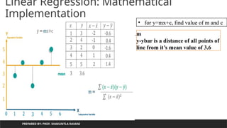
• 1. Find equation of line from
x and y values
• For that
• calculate mean of x and
mean of y:
mean(x)=(1+2+3+4+5)/5=3
mean(y)=(3+4+2+4+5)/
5=18/5=3.6
Plot mean point(3,3.6)
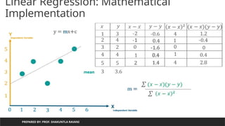
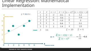
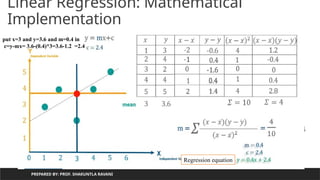
Using Regression equationcalculate
value of y from value of x
PREPARED BY: PROF. SHAKUNTLA RAVANI
m=0.4
c=2.4
y=0.4x+2.4
for given m=0.4 and &c=2.4
lets predict value for y using
x=[1,2,3,4,5]
x=1,y=0.4 *1+ 2.4 =2.8
x=2,y=0.4 *2+ 2.4 =3.2
x=3,y=0.4 *3+ 2.4 =3.6
x=4,y=0.4 *4+ 2.4 =4.0
x=5,y=0.4 *5+ 2.4 =4.4
18.
Using Regression equationcalculate
value of y from value of x
PREPARED BY: PROF. SHAKUNTLA RAVANI
m=0.4
c=2.4
y=0.4x+2.4
for given m=0.4 and &c=2.4
lets predict value for y using
x=[1,2,3,4,5]
x=1,y=0.4 *1+ 2.4 =2.8
x=2,y=0.4 *2+ 2.4 =3.2
x=3,y=0.4 *3+ 2.4 =3.6
x=4,y=0.4 *4+ 2.4 =4.0
x=5,y=0.4 *5+ 2.4 =4.4
19.
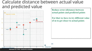
Calculate distance betweenactual value
and predicted value
PREPARED BY: PROF. SHAKUNTLA RAVANI
Reduce error (distance) between
actual points and predicted points
For that we have to try different value
of m to get closer to actual points
20.
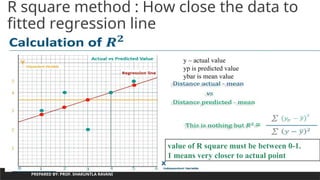
R square method: How close the data to
fitted regression line
PREPARED BY: PROF. SHAKUNTLA RAVANI
value of R square must be between 0-1.
1 means very closer to actual point
y – actual value
yp is predicted value
ybar is mean value
PREPARED BY: PROF.SHAKUNTLA RAVANI
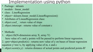
Implementation using python
• Package : sklearn
• module : linear_model
• class : LinerRegression
• object= sklearn.linear_model.LinearRegression()
• Attributes of LinearRegression class:
1. object.coef_ : returs value of slope
2. object.intercept : returns value of constant c
• Methods:
1. object.fit(N-dimension array X, array Y)
here value of x and y points will be passed to perform linear regression.
2. ypre=object.predict(x) : returns new value of y on bases of linear regression
equation y=mx+c, by applying value of m, x and c
3. object.score(x,y) : returns distance of actual points and predicted points-R2
24.
PREPARED BY: PROF.SHAKUNTLA RAVANI
Implementation using python
x=[1,2,3,4,5]
y=[3,4,2,4,5]
import pandas as pd
d={'X':x,'Y':y}
df=pd.DataFrame(d)
print(df)
from sklearn.linear_model import LinearRegression
X = df['X'].values.reshape(-1,1)
#the unspecified value is inferred to be original value
Y = df['Y'].values.reshape(-1,1)
h=LinearRegression()
h.fit(X,Y)
print(h.coef_) #value of m
print(h.intercept_)# value of c
ypre=h.predict(X)
print(ypre)
h.score(X,Y) #distance of actual points and predicted points
25.
PREPARED BY: PROF.SHAKUNTLA RAVANI
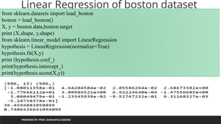
Linear Regression of boston dataset
from sklearn.datasets import load_boston
boston = load_boston()
X, y = boston.data,boston.target
print (X.shape, y.shape)
from sklearn.linear_model import LinearRegression
hypothesis = LinearRegression(normalize=True)
hypothesis.fit(X,y)
print (hypothesis.coef_)
print(hypothesis.intercept_)
print(hypothesis.score(X,y))
26.
PREPARED BY: PROF.SHAKUNTLA RAVANI
we print the value of the boston_dataset to understand what it contains. print(boston_dataset.keys()) gives
dict_keys(['data', 'target', 'feature_names', 'DESCR'])
•data: contains the information for various houses
•target: prices of the house
•feature_names: names of the features
•DESCR: describes the dataset
To know more about the features use boston_dataset.DESCR The description of all the features is given below:
CRIM: Per capital crime rate by town
ZN: Proportion of residential land zoned for lots over 25,000 sq. ft
INDUS: Proportion of non-retail business acres per town
CHAS: Charles River dummy variable (= 1 if tract bounds river; 0 otherwise)
NOX: Nitric oxide concentration (parts per 10 million)
RM: Average number of rooms per dwelling
AGE: Proportion of owner-occupied units built prior to 1940
DIS: Weighted distances to five Boston employment centers
RAD: Index of accessibility to radial highways
TAX: Full-value property tax rate per $10,000
PTRATIO: Pupil-teacher ratio by town
B: 1000(Bk — 0.63)², where Bk is the proportion of [people of African American descent] by town
LSTAT: Percentage of lower status of the population
MEDV: Median value of owner-occupied homes in $1000s
The prices of the house indicated by the variable MEDV is our target variable and the remaining are the feature
variables based on which we will predict the value of a house.
We will now load the data into a pandas dataframe using pd.DataFrame. We then print the first 5 rows of the data
using head()
27.
PREPARED BY: PROF.SHAKUNTLA RAVANI
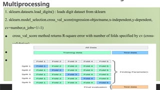
Multiprocessing
1. sklearn.datasets.load_digits() : loads digit dataset from sklearn
2. sklearn.model_selection.cross_val_score(regression-objectname,x-independent,y-dependent,
cv=number,n_jobs=1/-1)
• cross_val_score method returns R-square error with number of folds specified by cv (cross-
validation)
• cv=number of folds (groups of data) Example : cv=5
• jobs=1 – uniprocessor , -1 : multicore
28.
PREPARED BY: PROF.SHAKUNTLA RAVANI
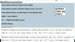
Execute code on multicore instead of single core-
Multiprocessing
from sklearn.datasets import load_digits
from sklearn.model_selection import cross_val_score
from sklearn.linear_model import LinearRegression
digits = load_digits()
X, y = digits.data,digits.target
print(X.shape)
print(y.shape)
l=LinearRegression()
single_core_learning = cross_val_score(l, X, y, cv=20, n_jobs=1)
#print(single_core_learning)
OUTPUT
(1797, 64)
(1797,)
29.
PREPARED BY: PROF.SHAKUNTLA RAVANI
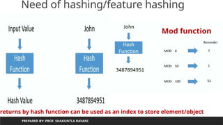
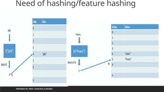
Need of hashing/feature hashing
Index is used to access element:
Array[3] will gives value4
When we do not want to worry about
Number of elements in advance :
30.
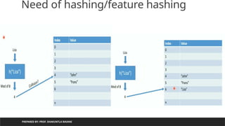
Need of hashing/featurehashing
PREPARED BY: PROF. SHAKUNTLA RAVANI
returns by hash function can be used as an index to store element/object
Mod function
31.
PREPARED BY: PROF.SHAKUNTLA RAVANI
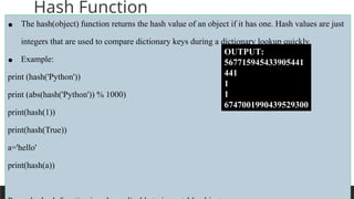
Hash Function
• The hash(object) function returns the hash value of an object if it has one. Hash values are just
integers that are used to compare dictionary keys during a dictionary lookup quickly.
• Example:
print (hash('Python'))
print (abs(hash('Python')) % 1000)
print(hash(1))
print(hash(True))
a='hello'
print(hash(a))
OUTPUT:
567715945433905441
441
1
1
6747001990439529300
32.
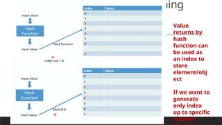
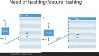
Need of hashing/featurehashing
PREPARED BY: PROF. SHAKUNTLA RAVANI
Value
returns by
hash
function can
be used as
an index to
store
element/obj
ect
If we want to
generate
only index
up to specific
number
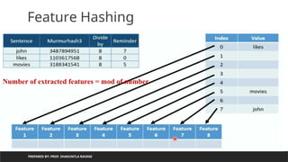
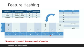
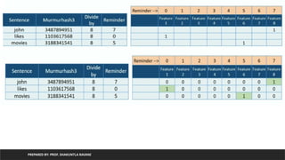
PREPARED BY: PROF.SHAKUNTLA RAVANI
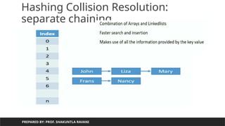
Hashing
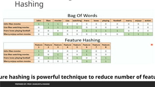
ure hashing is powerful technique to reduce number of featu
42.
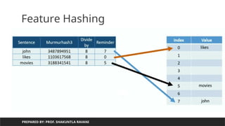
data science”
PREPARED BY:PROF. SHAKUNTLA RAVANI
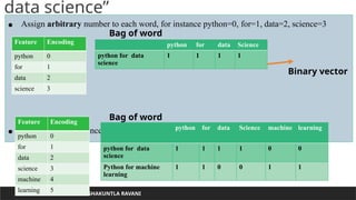
• Assign arbitrary number to each word, for instance python=0, for=1, data=2, science=3
• Add one more sentence : python for machine learning
Feature Encoding
python 0
for 1
data 2
science 3
python for data Science
python for data
science
1 1 1 1
Bag of word
Binary vector
Feature Encoding
python 0
for 1
data 2
science 3
machine 4
learning 5
python for data Science machine learning
python for data
science
1 1 1 1 0 0
Python for machine
learning
1 1 0 0 1 1
Bag of word
43.
PREPARED BY: PROF.SHAKUNTLA RAVANI
encoding
from sklearn.feature_extraction.text import *
bow=CountVectorizer()
bowm=bow.fit_transform(['python for data science','python for machine learning']).toarray()
print(bow.vocabulary_)
OUTPUT:
{'python': 4, 'for': 1, 'data': 0, 'science': 5, 'machine': 3, 'learning': 2}
python for data science
python for machine learning
data for
learning
machine
python
science
44.
PREPARED BY: PROF.SHAKUNTLA RAVANI
encoding
from sklearn.feature_extraction.text import *
bow=CountVectorizer()
bowm=bow.fit_transform(['python for data science','python for machine learning']).toarray()
bowm1=bow.transform(['new text has arrived']).toarray()
ry_)
OUTPUT:
{'python': 4, 'for': 1, 'data': 0, 'science': 5, 'machine': 3, 'learning': 2}
New text has arrived
data for
learning
machine
python
science
Limitations:
1. Require more storage if document is large (per feature-word one index occupied)
2. Optimally encodes text in matrix but once matrix generated, new text can not be
inserted
45.
PREPARED BY: PROF.SHAKUNTLA RAVANI
defined
string_1 = 'Python for data science'
string_2 = 'Python for machine learning'
def hashing_trick(input_string, vector_size=20):
feature_vector = [0] * vector_size
for word in input_string.split(' '):
index = abs(hash(word)) % vector_size
print('word is:',word,'original hash value',hash(word),'index is:',index)
feature_vector[index] = 1
46.
PREPARED BY: PROF.SHAKUNTLA RAVANI
defined
OUTPUT:
word is: Python original hash value -5119337540373521090 index is: 10
word is: for original hash value -5304979803602257784 index is: 4
word is: data original hash value -250754315164222072 index is: 12
word is: science original hash value -4211303434629928500 index is: 0
[1, 0, 0, 0, 1, 0, 0, 0, 0, 0, 1, 0, 1, 0, 0, 0, 0, 0, 0, 0]
word is: Python original hash value -5119337540373521090 index is: 10
word is: for original hash value -5304979803602257784 index is: 4
word is: machine original hash value 3675180801325909671 index is: 11
Remark : if vectorsize is small then many words overlap to same location in list
representing feature vector. To keep overlap minimum mod value should be large enough
47.
PREPARED BY: PROF.SHAKUNTLA RAVANI
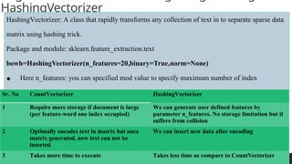
HashingVectorizer
HashingVectorizer: A class that rapidly transforms any collection of text in to separate sparse data
matrix using hashing trick.
Package and module: sklearn.feature_extraction.text
bowh=HashingVectorizer(n_features=20,binary=True,norm=None)
• Here n_features: you can specified mod value to specify maximum number of index
generation. For example: 20 means indexes will be 0-19 to store words(features)
• Binary=True : binary encoding – If feature is available then 1 else 0
Sr. No CountVectorizer HashingVectorizer
1 Require more storage if document is large
(per feature-word one index occupied)
We can generate user defined features by
parameter n_features. No storage limitation but it
suffers from collision
2 Optimally encodes text in matrix but once
matrix generated, new text can not be
inserted
We can insert new data after encoding
3 Takes more time to execute Takes less time as compare to CountVectorizer
PREPARED BY: PROF.SHAKUNTLA RAVANI
HashingVectorizer
from sklearn.feature_extraction.text import HashingVectorizer, CountVectorizer
bowh = HashingVectorizer(n_features=20, binary=True, norm=None)
bowc = CountVectorizer()
texts = ['Python for data science','Python for machine learning']
50.
PREPARED BY: PROF.SHAKUNTLA RAVANI
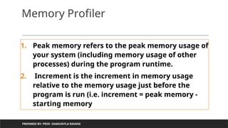
Memory Profiler
Useful to find out memory usage (space complexity) of particular statement of program
Package: memory_profiler
• Command to install (type on Jupyter Notebook)
1. import sys
2. ! (sys.executable) –m pip install memory_profiler
After installation completes, type below command on jupyter Notebook
3. %load memory_profiler
For find out memory requirement for hashing matrix give use magic function %memit as below:
%memit bowhm = bowh.fit_transform(texts).toarray()
Memory Profiler
1. Peakmemory refers to the peak memory usage of
your system (including memory usage of other
processes) during the program runtime.
2. Increment is the increment in memory usage
relative to the memory usage just before the
program is run (i.e. increment = peak memory -
starting memory
PREPARED BY: PROF. SHAKUNTLA RAVANI
Exploratory Data Analysis(EDA)
PREPARED BY: PROF. SHAKUNTLA RAVANI
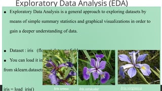
• Exploratory Data Analysis is a general approach to exploring datasets by
means of simple summary statistics and graphical visualizations in order to
gain a deeper understanding of data.
• Dataset : iris (flower) dataset of sklearn
• You can load it in python program using:
from sklearn.datasets import load_iris
iris = load_iris() Iris setosa Iris versicolor Iris virginica
55.
Exploratory Data Analysis(EDA)
PREPARED BY: PROF. SHAKUNTLA RAVANI
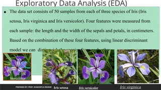
• The data set consists of 50 samples from each of three species of Iris (Iris
setosa, Iris virginica and Iris versicolor). Four features were measured from
each sample: the length and the width of the sepals and petals, in centimeters.
Based on the combination of these four features, using linear discriminant
model we can distinguish the species from each other.
Iris setosa Iris versicolor Iris virginica
PREPARED BY: PROF.SHAKUNTLA RAVANI
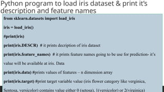
Python program to load iris dataset & print it’s
description and feature names
from sklearn.datasets import load_iris
iris = load_iris()
#print(iris)
print(iris.DESCR) # it prints decription of iris dataset
print(iris.feature_names) # it prints feature names going to be use for prediction- it’s
value will be available at iris. Data
print(iris.data) #prints values of features – n dimension array
print(iris.target) #print target variable value (iris flower category like verginica,
Sentosa, versicolor) contains value either 0 (setosa), 1(versicolor) or 2(virginica)
58.
PREPARED BY: PROF.SHAKUNTLA RAVANI
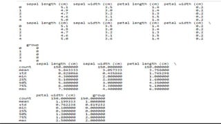
Generate dataframe from iris dataset by using data attribute
and target attribute and print statistical analysis------version 1
from sklearn.datasets import load_iris
import pandas as pd
iris=load_iris()
df=pd.DataFrame(iris.data, columns=iris.feature_names)
print(df.head())
df['group']=iris.target # adding flower type in form of 0,1,2
print(df.head())
print(df.describe())
PREPARED BY: PROF.SHAKUNTLA RAVANI
print flower type in string instead of category code
from sklearn.datasets import load_iris
import pandas as pd
iris=load_iris()
print(iris.target)
for k in iris.target:
print(iris.target_names[k])
61.
PREPARED BY: PROF.SHAKUNTLA RAVANI
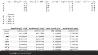
Generate dataframe from iris dataset by using data attribute and
target attribute and print statistical analysis------version 2
considering as target as a category of flower (data in from of string)
from sklearn.datasets import load_iris
import pandas as pd
iris=load_iris()
df=pd.DataFrame(iris.data, columns=iris.feature_names)
df['group']=pd.Series([iris.target_names[k] for k in iris.target], dtype='category')
print(df.head())
df.describe()
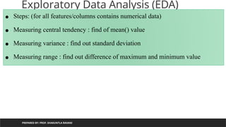
Exploratory Data Analysis(EDA)
PREPARED BY: PROF. SHAKUNTLA RAVANI
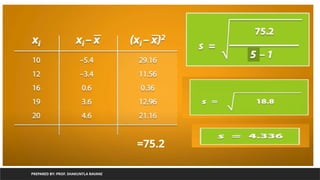
• Steps: (for all features/columns contains numerical data)
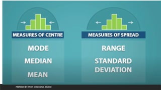
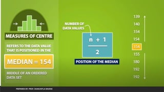
• Measuring central tendency : find of mean() value
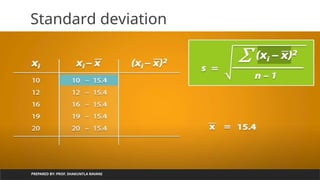
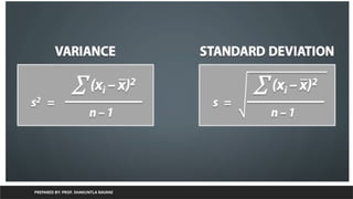
• Measuring variance : find out standard deviation
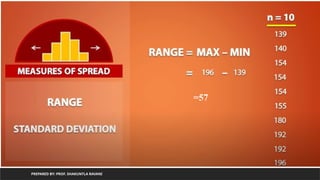
• Measuring range : find out difference of maximum and minimum value
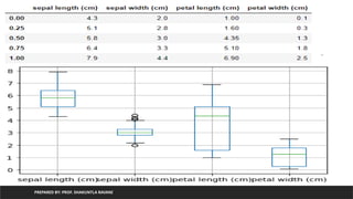
plot of iris
PREPAREDBY: PROF. SHAKUNTLA RAVANI
from sklearn.datasets import load_iris
import pandas as pd
iris=load_iris()
df=pd.DataFrame(iris.data, columns=iris.feature_names)
df['group']=pd.Series([iris.target_names[k] for k in iris.target],dtype='category’)
print(df.quantile([0,0.25,0.50,0.75,1]))
import matplotlib.pyplot as plt
df.boxplot()
plt.show()
PREPARED BY: PROF.SHAKUNTLA RAVANI
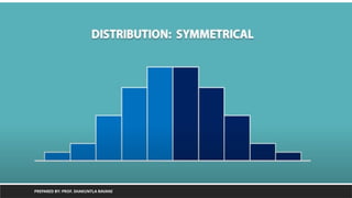
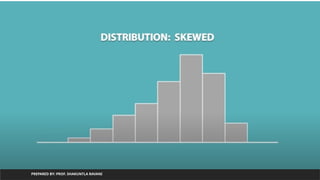
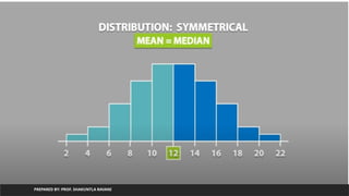
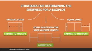
Skewness
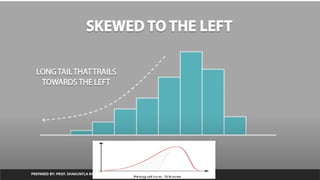
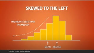
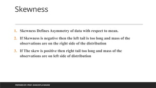
1. Skewness Defines Asymmetry of data with respect to mean.
2. If Skewness is negative then the left tail is too long and mass of the
observations are on the right side of the distribution
3. If The skew is positive then right tail too long and mass of the
observations are on left side of distribution
118.
PREPARED BY: PROF.SHAKUNTLA RAVANI
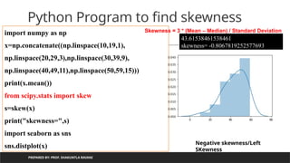
Python Program to find skewness
import numpy as np
x=np.concatenate((np.linspace(10,19,1),
np.linspace(20,29,3),np.linspace(30,39,9),
np.linspace(40,49,11),np.linspace(50,59,15)))
print(x.mean())
from scipy.stats import skew
s=skew(x)
print("skewness=",s)
import seaborn as sns
sns.distplot(x)
43.61538461538461
skewness= -0.8067819252577693
Negative skewness/Left
SKewness
Skewness = 3 * (Mean – Median) / Standard Deviation
119.
PREPARED BY: PROF.SHAKUNTLA RAVANI
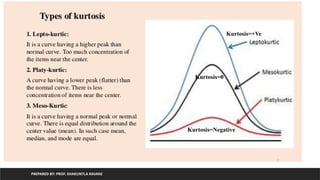
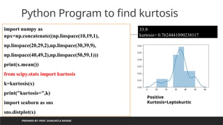
Kurtosis
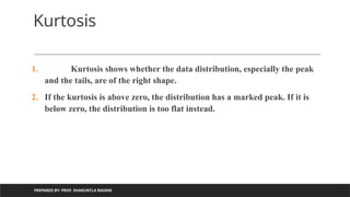
1. Kurtosis shows whether the data distribution, especially the peak
and the tails, are of the right shape.
2. If the kurtosis is above zero, the distribution has a marked peak. If it is
below zero, the distribution is too flat instead.
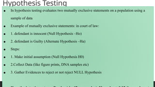
Hypothesis Testing
PREPARED BY:PROF. SHAKUNTLA RAVANI
• In hypothesis testing evaluates two mutually exclusive statements on a population using a
sample of data
• Example of mutually exclusive statements: in court of law:
• 1. defendant is innocent (Null Hypothesis –Ho)
• 2. defendant is Guilty (Alternate Hypothesis –Ha)
• Steps:
• 1. Make initial assumption (Null Hypothesis H0)
• 2.Collect Data (like figure prints, DNA samples etc)
• 3. Gather Evidences to reject or not reject NULL Hypothesis
137.
PREPARED BY: PROF.SHAKUNTLA RAVANI
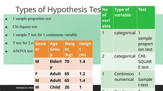
• 1 sample proportion test
• Chi-Square test
• 1 sample T test for 1 continuous variable
• T test for 2 continuous variable
• ANOVA test for more than 2 continuous variables
Types of Hypothesis Testing
No
of
vari
able
Type of
variable
Test
1 categorical 1
sample
proport
ion test
2 categorical CHI-
SQUAR
E test
1 Continous
numerical
1
Sample
t-test
Gend
er
Age
Grou
p
Weig
ht
(kg)
Heigh
t
(m)
M Elderl
y
70 1.4
F Adult 65 1.2
M Adult 65 1.4
M Child 20 1
138.
PREPARED BY: PROF.SHAKUNTLA RAVANI
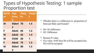
Types of Hypothesis Testing: 1 sample
Proportion test
Gend
er
Age
Grou
p
Weig
ht
Heigh
t
M Elderl
y
70 1.4
F Adult 65 1.2
M Adult 65 1.4
M Child 20 1
F Adult 75 1.3
M Elderl
y
80 1.3
• Whether there is a difference in proportion of
between Male and Female?
• Ho: No difference
• H1: Difference
• Returns P-value
• If p value >0.05 then Ho will be accepted else
HA will be accepted
139.
PREPARED BY: PROF.SHAKUNTLA RAVANI
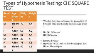
Types of Hypothesis Testing: CHI SQUARE
TEST
Gend
er
Age
Grou
p
Weig
ht
Heigh
t
M Elderl
y
70 1.4
F Adult 65 1.2
M Adult 65 1.4
M Child 20 1
F Adult 75 1.3
M Elderl
y
80 1.3
• Whether there is a difference in proportion of
between Male and Female bases on Age group
?
• Ho: No difference
• H1: Difference
• Returns P-value
• If p value >0.05 then Ho will be accepted else
HA will be accepted
PREPARED BY: PROF.SHAKUNTLA RAVANI
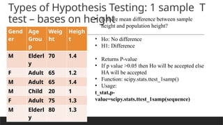
Types of Hypothesis Testing: 1 sample T
test – bases on height
Gend
er
Age
Grou
p
Weig
ht
Heigh
t
M Elderl
y
70 1.4
F Adult 65 1.2
M Adult 65 1.4
M Child 20 1
F Adult 75 1.3
M Elderl
y
80 1.3
• Is there mean difference between sample
height and population height?
• Ho: No difference
• H1: Difference
• Returns P-value
• If p value >0.05 then Ho will be accepted else
HA will be accepted
• Function: scipy.stats.ttest_1samp()
• Usage:
t_stat,p-
value=scipy.stats.ttest_1samp(sequence)
142.
variable)
PREPARED BY: PROF.SHAKUNTLA RAVANI
ages=[10,20,35,50,28,40,55,18,16,55,30,25,43,18,30,28,14,24,16,17,32,35,26,27,65,18,43,23,21,20,19,70]
print(len(ages))
import numpy as np
ages_mean=np.mean(ages)
print(ages_mean)
## Lets take sample
sample_size=10
age_sample=np.random.choice(ages,sample_size)
print(age_sample)
from scipy.stats import ttest_1samp
ttest,p_value=ttest_1samp(age_sample,30)
print(p_value)
32
30.34375
[18 40 16 50 28 27 50 30 30 55]
0.33568006273592693
we are accepting null hypothesis
new p value 1.0
143.
flower groups
PREPARED BY:PROF. SHAKUNTLA RAVANI
from scipy.stats import ttest_ind
from sklearn.datasets import load_iris
import pandas as pd
iris=load_iris()
df=pd.DataFrame(iris.data, columns=iris.feature_names)
df['group']=pd.Series([iris.target_names[k] for k in iris.target],dtype='category')
group0 = df['group'] == 'setosa'
group1 = df['group'] == 'versicolor'
group2 = df['group'] == 'virginica'
t,pvalue=ttest_ind(df['petal length (cm)'][group0],df['petal length (cm)'][group1])
< 0.05, Null hypothesis rejected
Means mean difference is there between
group 0 and group 1
Function: scipy.stats.ttest_ind(var1, var2)
It returs p value and statistical difference
difference
PREPARED BY: PROF.SHAKUNTLA RAVANI
from scipy.stats import f_oneway
from sklearn.datasets import load_iris
import pandas as pd
iris=load_iris()
df=pd.DataFrame(iris.data, columns=iris.feature_names)
df['group']=pd.Series([iris.target_names[k] for k in iris.target],dtype='category')
group0 = df['group'] == 'setosa'
group1 = df['group'] == 'versicolor'
group2 = df['group'] == 'virginica'
f,pvalue=f_oneway(df['petal length (cm)'][group0],df['petal length (cm)'][group1],df['petal length
< 0.05, Null hypothesis rejected
Means mean difference is there between
group 0, group 1 and group 2
Function: scipy.stats.f_oneway(group1, group2,group3,...)
It returs p value and statistical difference
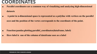
COORDINATES
PREPARED BY: PROF.SHAKUNTLA RAVANI
• Parallel coordinates are a common way of visualizing and analyzing high-dimensional
datasets
• A point in n-dimensional space is represented as a polyline with vertices on the parallel
axes and the position of the vertex corresponds to the coordinate of the point.
• Function:pandas.plotting.parallel_coordinates(dataframe, label)
• Here label is one of the column of dataframe uses as a label
148.
dataframe
PREPARED BY: PROF.SHAKUNTLA RAVANI
from pandas.plotting import parallel_coordinates
from sklearn.datasets import load_iris
import pandas as pd
iris=load_iris()
df=pd.DataFrame(iris.data,
columns=iris.feature_names)
df['label']=pd.Series( [iris.target_names[k] for k in
iris.target],dtype='category')
df['group']=iris.target
pl=parallel_coordinates(df,'label')
histogram
PREPARED BY: PROF.SHAKUNTLA RAVANI
• Function for density plot:
• pandas.DataFrame.plot(kind=‘density’)
• Or
• pandas.DataFrame[‘column-name’].plot(kind=‘density’)
• Function for histogram for specific column of dataframe/whole dataframe
• pandas.DataFrame.plot(kind=‘hist’)
151.
dataframe
PREPARED BY: PROF.SHAKUNTLA RAVANI
from sklearn.datasets import load_iris
import pandas as pd
iris=load_iris()
df=pd.DataFrame(iris.data,
columns=iris.feature_names)
df['group']=pd.Series([iris.target_names[k] for k in
iris.target],dtype='category')
df.plot(kind='density')
df.plot(kind='hist')
Function for scatterplot
PREPARED BY: PROF. SHAKUNTLA RAVANI
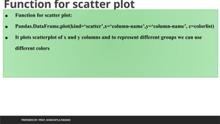
• Function for scatter plot:
• Pandas.DataFrame.plot(kind=‘scatter’,x=‘column-name’,y=‘column-name’, c=colorlist)
• It plots scatterplot of x and y columns and to represent different groups we can use
different colors
154.
Function for scatterplot
PREPARED BY: PROF. SHAKUNTLA RAVANI
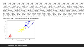
from sklearn.datasets import load_iris
import pandas as pd
iris=load_iris()
df=pd.DataFrame(iris.data, columns=iris.feature_names)
df['group']=iris.target
pelette={0:'red',1:'yellow',2:'blue'}
color=[pelette[k] for k in df['group']]
print(color)
df.plot(kind='scatter',x='petal length (cm)',y='petal width (cm)',c=color)
Function for scattermatrix
PREPARED BY: PROF. SHAKUNTLA RAVANI
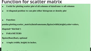
• Useful for plotting scatter plot of all columns of dataframe vs all columns
• At diagonal position we can plot either histogram or density plot
• Function:
pandas.plotting.scatter_matrix(dataframename,figsize(width,height),color=colors,
diagonal=‘hist/kde’)
• PARAMETERS
figsize(float,float), optional
• A tuple (width, height) in inches.
157.
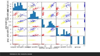
Scatter matrix forall columns->all
columns of iris
PREPARED BY: PROF. SHAKUNTLA RAVANI
from pandas.plotting import scatter_matrix
from sklearn.datasets import load_iris
import pandas as pd
iris=load_iris()
df=pd.DataFrame(iris.data, columns=iris.feature_names)
df['group']=iris.target
pelette={0:'red',1:'yellow',2:'blue'}
colorlist=[pelette[k] for k in df['group']]
scatter_matrix(df,figsize=(6,6),color=colorlist,diagonal='hist')
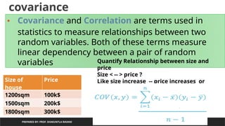
covariance
PREPARED BY: PROF.SHAKUNTLA RAVANI
• Covariance and Correlation are terms used in
statistics to measure relationships between two
random variables. Both of these terms measure
linear dependency between a pair of random
variables
Size of
house
Price
1200sqm 100k$
1500sqm 200k$
1800sqm 300k$
Quantify Relationship between size and
price
Size < -- > price ?
Like size increase -- price increases or
Size decreases ----price decreases
161.
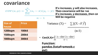
covariance
PREPARED BY: PROF.SHAKUNTLA RAVANI
Size of
house
Price
1200sqm 100k$
1500sqm 200k$
1800sqm 300k$
• Cov(X,X)=∑
𝑖=1
𝑛
(𝑥 −𝑥𝑏𝑎𝑟)(𝑥−𝑥𝑏𝑎𝑟)
𝑛−1
If x increases, y will also increases,
Then covariance will be +ve
If x increases, y decreases, then cov
Will be negative
Function:
pandas.DataFrameob.c
ov()
162.
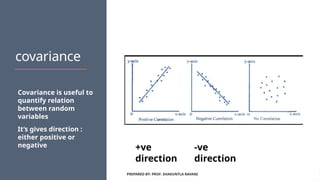
covariance
Covariance is usefulto
quantify relation
between random
variables
It’s gives direction :
either positive or
negative
PREPARED BY: PROF. SHAKUNTLA RAVANI
-ve
direction
+ve
direction
163.
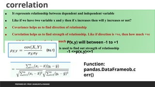
correlation
PREPARED BY: PROF.SHAKUNTLA RAVANI
• It represents relationship between dependent and independent variable
• Like if we have two variable x and y then if x increases then will y increases or not?
• Covariance helps us to find direction of relationship
• Correlation helps us to find strength of relationship. Like if direction is +ve, then how much +ve
and if direction is –ve then how much -ve
• Perason’s correlation coefficient is used to find out strength of relationship
P(x,y) will between -1 to +1
-1 <=p(x,y)<=1
Function:
pandas.DataFrameob.c
orr()
164.
PREPARED BY: PROF.SHAKUNTLA RAVANI
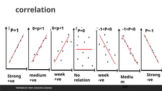
correlation
P=1
P=1
0<p<1
0<p<1 P=0
P=0
-1<P<0
-1<P<0 -1<P<0 P=-1
Strong
+ve
Strong
-ve
medium
+ve
week
+ve
No
relation
week
-ve
Mediu
m
-ve
165.
Python program toprint covariance of all columns
with respect to all other columns of iris
PREPARED BY: PROF. SHAKUNTLA RAVANI
from sklearn.datasets import load_iris
import pandas as pd
iris=load_iris()
df=pd.DataFrame(iris.data, columns=iris.feature_names)
df['group']=iris.target
df.cov()
166.
Python program toprint pearson’s correlation coefficient
of all columns with respect to all other columns of iris
PREPARED BY: PROF. SHAKUNTLA RAVANI
from sklearn.datasets import load_iris
import pandas as pd
iris=load_iris()
df=pd.DataFrame(iris.data, columns=iris.feature_names)
df['group']=iris.target
df.corr()
167.
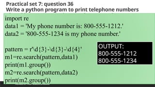
Practical set 7:question 36
Write a python program to print telephone numbers
placed in sentences using regular expressions
PREPARED BY: PROF. SHAKUNTLA RAVANI
import re
data1 = 'My phone number is: 800-555-1212.'
data2 = '800-555-1234 is my phone number.'
pattern = r'd{3}-d{3}-d{4}'
m1=re.search(pattern,data1)
print(m1.group())
m2=re.search(pattern,data2)
print(m2.group())
OUTPUT:
800-555-1212
800-555-1234
168.
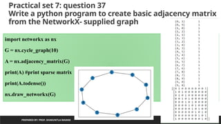
Practical set 7:question 37
Write a python program to create basic adjacency matrix
from the NetworkX- supplied graph
PREPARED BY: PROF. SHAKUNTLA RAVANI
import networkx as nx
G = nx.cycle_graph(10)
A = nx.adjacency_matrix(G)
print(A) #print sparse matrix
print(A.todense())
nx.draw_networkx(G)
169.
Practical set 7:question 38
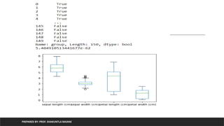
Write a python program to create applied visualization for
EDA using boxplots and perform t-tests.
PREPARED BY: PROF. SHAKUNTLA RAVANI
from sklearn.datasets import load_iris
import pandas as pd
iris=load_iris()
df=pd.DataFrame(iris.data,columns=iris.feature_names)
df['group']=pd.Series([iris.target_names[k] for k in iris.target],dtype='category')
df.plot(kind='box')
group1=df['group']=='setosa'
group2=df['group']=='versicolor'
print(group1)


![Using Regression equation calculate
value of y from value of x
PREPARED BY: PROF. SHAKUNTLA RAVANI
m=0.4
c=2.4
y=0.4x+2.4
for given m=0.4 and &c=2.4
lets predict value for y using
x=[1,2,3,4,5]
x=1,y=0.4 *1+ 2.4 =2.8
x=2,y=0.4 *2+ 2.4 =3.2
x=3,y=0.4 *3+ 2.4 =3.6
x=4,y=0.4 *4+ 2.4 =4.0
x=5,y=0.4 *5+ 2.4 =4.4](https://image.slidesharecdn.com/unit-5-250628061527-8444998e/85/unit-5-Data-Wrandling-weightage-marks-pptx-17-320.jpg)
![Using Regression equation calculate
value of y from value of x
PREPARED BY: PROF. SHAKUNTLA RAVANI
m=0.4
c=2.4
y=0.4x+2.4
for given m=0.4 and &c=2.4
lets predict value for y using
x=[1,2,3,4,5]
x=1,y=0.4 *1+ 2.4 =2.8
x=2,y=0.4 *2+ 2.4 =3.2
x=3,y=0.4 *3+ 2.4 =3.6
x=4,y=0.4 *4+ 2.4 =4.0
x=5,y=0.4 *5+ 2.4 =4.4](https://image.slidesharecdn.com/unit-5-250628061527-8444998e/85/unit-5-Data-Wrandling-weightage-marks-pptx-18-320.jpg)
![PREPARED BY: PROF. SHAKUNTLA RAVANI
Implementation using python
x=[1,2,3,4,5]
y=[3,4,2,4,5]
import pandas as pd
d={'X':x,'Y':y}
df=pd.DataFrame(d)
print(df)
from sklearn.linear_model import LinearRegression
X = df['X'].values.reshape(-1,1)
#the unspecified value is inferred to be original value
Y = df['Y'].values.reshape(-1,1)
h=LinearRegression()
h.fit(X,Y)
print(h.coef_) #value of m
print(h.intercept_)# value of c
ypre=h.predict(X)
print(ypre)
h.score(X,Y) #distance of actual points and predicted points](https://image.slidesharecdn.com/unit-5-250628061527-8444998e/85/unit-5-Data-Wrandling-weightage-marks-pptx-24-320.jpg)
![PREPARED BY: PROF. SHAKUNTLA RAVANI
we print the value of the boston_dataset to understand what it contains. print(boston_dataset.keys()) gives
dict_keys(['data', 'target', 'feature_names', 'DESCR'])
•data: contains the information for various houses
•target: prices of the house
•feature_names: names of the features
•DESCR: describes the dataset
To know more about the features use boston_dataset.DESCR The description of all the features is given below:
CRIM: Per capital crime rate by town
ZN: Proportion of residential land zoned for lots over 25,000 sq. ft
INDUS: Proportion of non-retail business acres per town
CHAS: Charles River dummy variable (= 1 if tract bounds river; 0 otherwise)
NOX: Nitric oxide concentration (parts per 10 million)
RM: Average number of rooms per dwelling
AGE: Proportion of owner-occupied units built prior to 1940
DIS: Weighted distances to five Boston employment centers
RAD: Index of accessibility to radial highways
TAX: Full-value property tax rate per $10,000
PTRATIO: Pupil-teacher ratio by town
B: 1000(Bk — 0.63)², where Bk is the proportion of [people of African American descent] by town
LSTAT: Percentage of lower status of the population
MEDV: Median value of owner-occupied homes in $1000s
The prices of the house indicated by the variable MEDV is our target variable and the remaining are the feature
variables based on which we will predict the value of a house.
We will now load the data into a pandas dataframe using pd.DataFrame. We then print the first 5 rows of the data
using head()](https://image.slidesharecdn.com/unit-5-250628061527-8444998e/85/unit-5-Data-Wrandling-weightage-marks-pptx-26-320.jpg)
![PREPARED BY: PROF. SHAKUNTLA RAVANI
Need of hashing/feature hashing
Index is used to access element:
Array[3] will gives value4
When we do not want to worry about
Number of elements in advance :](https://image.slidesharecdn.com/unit-5-250628061527-8444998e/85/unit-5-Data-Wrandling-weightage-marks-pptx-29-320.jpg)
![PREPARED BY: PROF. SHAKUNTLA RAVANI
encoding
from sklearn.feature_extraction.text import *
bow=CountVectorizer()
bowm=bow.fit_transform(['python for data science','python for machine learning']).toarray()
print(bow.vocabulary_)
OUTPUT:
{'python': 4, 'for': 1, 'data': 0, 'science': 5, 'machine': 3, 'learning': 2}
python for data science
python for machine learning
data for
learning
machine
python
science](https://image.slidesharecdn.com/unit-5-250628061527-8444998e/85/unit-5-Data-Wrandling-weightage-marks-pptx-43-320.jpg)
![PREPARED BY: PROF. SHAKUNTLA RAVANI
encoding
from sklearn.feature_extraction.text import *
bow=CountVectorizer()
bowm=bow.fit_transform(['python for data science','python for machine learning']).toarray()
bowm1=bow.transform(['new text has arrived']).toarray()
ry_)
OUTPUT:
{'python': 4, 'for': 1, 'data': 0, 'science': 5, 'machine': 3, 'learning': 2}
New text has arrived
data for
learning
machine
python
science
Limitations:
1. Require more storage if document is large (per feature-word one index occupied)
2. Optimally encodes text in matrix but once matrix generated, new text can not be
inserted](https://image.slidesharecdn.com/unit-5-250628061527-8444998e/85/unit-5-Data-Wrandling-weightage-marks-pptx-44-320.jpg)
![PREPARED BY: PROF. SHAKUNTLA RAVANI
defined
string_1 = 'Python for data science'
string_2 = 'Python for machine learning'
def hashing_trick(input_string, vector_size=20):
feature_vector = [0] * vector_size
for word in input_string.split(' '):
index = abs(hash(word)) % vector_size
print('word is:',word,'original hash value',hash(word),'index is:',index)
feature_vector[index] = 1](https://image.slidesharecdn.com/unit-5-250628061527-8444998e/85/unit-5-Data-Wrandling-weightage-marks-pptx-45-320.jpg)
![PREPARED BY: PROF. SHAKUNTLA RAVANI
defined
OUTPUT:
word is: Python original hash value -5119337540373521090 index is: 10
word is: for original hash value -5304979803602257784 index is: 4
word is: data original hash value -250754315164222072 index is: 12
word is: science original hash value -4211303434629928500 index is: 0
[1, 0, 0, 0, 1, 0, 0, 0, 0, 0, 1, 0, 1, 0, 0, 0, 0, 0, 0, 0]
word is: Python original hash value -5119337540373521090 index is: 10
word is: for original hash value -5304979803602257784 index is: 4
word is: machine original hash value 3675180801325909671 index is: 11
Remark : if vectorsize is small then many words overlap to same location in list
representing feature vector. To keep overlap minimum mod value should be large enough](https://image.slidesharecdn.com/unit-5-250628061527-8444998e/85/unit-5-Data-Wrandling-weightage-marks-pptx-46-320.jpg)
![PREPARED BY: PROF. SHAKUNTLA RAVANI
HashingVectorizer
from sklearn.feature_extraction.text import *
bowh = HashingVectorizer(n_features=20, binary=True,norm=None)
bowhm = bowh.fit_transform(['Python for data science','Python for machine
learning']).toarray()
print(bowhm)
bowhmn=bowh.transform(['new text has inserted']).toarray()
print(bowhmn)
OUTPUT:
[[0. 0. 0. 1. 0. 1. 0. 0. 0. 0. 0. 0. 0. 1. 0. 1. 0. 0. 0. 0.]
[0. 0. 1. 1. 1. 1. 0. 0. 0. 0. 0. 0. 0. 0. 0. 0. 0. 0. 0. 0.]]
[[1. 0. 0. 1. 0. 0. 0. 0. 0. 0. 0. 0. 1. 0. 1. 0. 0. 0. 0. 0.]]](https://image.slidesharecdn.com/unit-5-250628061527-8444998e/85/unit-5-Data-Wrandling-weightage-marks-pptx-48-320.jpg)
![PREPARED BY: PROF. SHAKUNTLA RAVANI
HashingVectorizer
from sklearn.feature_extraction.text import HashingVectorizer, CountVectorizer
bowh = HashingVectorizer(n_features=20, binary=True, norm=None)
bowc = CountVectorizer()
texts = ['Python for data science','Python for machine learning']](https://image.slidesharecdn.com/unit-5-250628061527-8444998e/85/unit-5-Data-Wrandling-weightage-marks-pptx-49-320.jpg)


![PREPARED BY: PROF. SHAKUNTLA RAVANI
Generate dataframe from iris dataset by using data attribute
and target attribute and print statistical analysis------version 1
from sklearn.datasets import load_iris
import pandas as pd
iris=load_iris()
df=pd.DataFrame(iris.data, columns=iris.feature_names)
print(df.head())
df['group']=iris.target # adding flower type in form of 0,1,2
print(df.head())
print(df.describe())](https://image.slidesharecdn.com/unit-5-250628061527-8444998e/85/unit-5-Data-Wrandling-weightage-marks-pptx-58-320.jpg)
![PREPARED BY: PROF. SHAKUNTLA RAVANI
print flower type in string instead of category code
from sklearn.datasets import load_iris
import pandas as pd
iris=load_iris()
print(iris.target)
for k in iris.target:
print(iris.target_names[k])](https://image.slidesharecdn.com/unit-5-250628061527-8444998e/85/unit-5-Data-Wrandling-weightage-marks-pptx-60-320.jpg)
![PREPARED BY: PROF. SHAKUNTLA RAVANI
Generate dataframe from iris dataset by using data attribute and
target attribute and print statistical analysis------version 2
considering as target as a category of flower (data in from of string)
from sklearn.datasets import load_iris
import pandas as pd
iris=load_iris()
df=pd.DataFrame(iris.data, columns=iris.feature_names)
df['group']=pd.Series([iris.target_names[k] for k in iris.target], dtype='category')
print(df.head())
df.describe()](https://image.slidesharecdn.com/unit-5-250628061527-8444998e/85/unit-5-Data-Wrandling-weightage-marks-pptx-61-320.jpg)


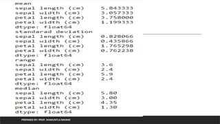
![iris
PREPARED BY: PROF. SHAKUNTLA RAVANI
from sklearn.datasets import load_iris
import pandas as pd
iris=load_iris()
df=pd.DataFrame(iris.data, columns=iris.feature_names)
df['group']=pd.Series([iris.target_names[k] for k in iris.target],dtype='category')
print(df.head())
print('mean')
print(df.mean())
print('standarad deviation')
print(df.std())](https://image.slidesharecdn.com/unit-5-250628061527-8444998e/85/unit-5-Data-Wrandling-weightage-marks-pptx-83-320.jpg)


![plot of iris
PREPARED BY: PROF. SHAKUNTLA RAVANI
from sklearn.datasets import load_iris
import pandas as pd
iris=load_iris()
df=pd.DataFrame(iris.data, columns=iris.feature_names)
df['group']=pd.Series([iris.target_names[k] for k in iris.target],dtype='category’)
print(df.quantile([0,0.25,0.50,0.75,1]))
import matplotlib.pyplot as plt
df.boxplot()
plt.show()](https://image.slidesharecdn.com/unit-5-250628061527-8444998e/85/unit-5-Data-Wrandling-weightage-marks-pptx-107-320.jpg)


![group
PREPARED BY: PROF. SHAKUNTLA RAVANI
from sklearn.datasets import load_iris
import pandas as pd
iris=load_iris()
df=pd.DataFrame(iris.data, columns=iris.feature_names)
df['group']=pd.Series([iris.target_names[k] for k in iris.target],dtype='category')
group0 = df['group'] == 'setosa'
print(group0.head())
group1 = df['group'] == 'versicolor'
group2 = df['group'] == 'virginica'
print('variance of geoup 0 is',df['petal length (cm)'][group0].var())](https://image.slidesharecdn.com/unit-5-250628061527-8444998e/85/unit-5-Data-Wrandling-weightage-marks-pptx-134-320.jpg)

![variable)
PREPARED BY: PROF. SHAKUNTLA RAVANI
ages=[10,20,35,50,28,40,55,18,16,55,30,25,43,18,30,28,14,24,16,17,32,35,26,27,65,18,43,23,21,20,19,70]
print(len(ages))
import numpy as np
ages_mean=np.mean(ages)
print(ages_mean)
## Lets take sample
sample_size=10
age_sample=np.random.choice(ages,sample_size)
print(age_sample)
from scipy.stats import ttest_1samp
ttest,p_value=ttest_1samp(age_sample,30)
print(p_value)
32
30.34375
[18 40 16 50 28 27 50 30 30 55]
0.33568006273592693
we are accepting null hypothesis
new p value 1.0](https://image.slidesharecdn.com/unit-5-250628061527-8444998e/85/unit-5-Data-Wrandling-weightage-marks-pptx-142-320.jpg)
![flower groups
PREPARED BY: PROF. SHAKUNTLA RAVANI
from scipy.stats import ttest_ind
from sklearn.datasets import load_iris
import pandas as pd
iris=load_iris()
df=pd.DataFrame(iris.data, columns=iris.feature_names)
df['group']=pd.Series([iris.target_names[k] for k in iris.target],dtype='category')
group0 = df['group'] == 'setosa'
group1 = df['group'] == 'versicolor'
group2 = df['group'] == 'virginica'
t,pvalue=ttest_ind(df['petal length (cm)'][group0],df['petal length (cm)'][group1])
< 0.05, Null hypothesis rejected
Means mean difference is there between
group 0 and group 1
Function: scipy.stats.ttest_ind(var1, var2)
It returs p value and statistical difference](https://image.slidesharecdn.com/unit-5-250628061527-8444998e/85/unit-5-Data-Wrandling-weightage-marks-pptx-143-320.jpg)
![difference
PREPARED BY: PROF. SHAKUNTLA RAVANI
from scipy.stats import f_oneway
from sklearn.datasets import load_iris
import pandas as pd
iris=load_iris()
df=pd.DataFrame(iris.data, columns=iris.feature_names)
df['group']=pd.Series([iris.target_names[k] for k in iris.target],dtype='category')
group0 = df['group'] == 'setosa'
group1 = df['group'] == 'versicolor'
group2 = df['group'] == 'virginica'
f,pvalue=f_oneway(df['petal length (cm)'][group0],df['petal length (cm)'][group1],df['petal length
< 0.05, Null hypothesis rejected
Means mean difference is there between
group 0, group 1 and group 2
Function: scipy.stats.f_oneway(group1, group2,group3,...)
It returs p value and statistical difference](https://image.slidesharecdn.com/unit-5-250628061527-8444998e/85/unit-5-Data-Wrandling-weightage-marks-pptx-145-320.jpg)

![dataframe
PREPARED BY: PROF. SHAKUNTLA RAVANI
from pandas.plotting import parallel_coordinates
from sklearn.datasets import load_iris
import pandas as pd
iris=load_iris()
df=pd.DataFrame(iris.data,
columns=iris.feature_names)
df['label']=pd.Series( [iris.target_names[k] for k in
iris.target],dtype='category')
df['group']=iris.target
pl=parallel_coordinates(df,'label')](https://image.slidesharecdn.com/unit-5-250628061527-8444998e/85/unit-5-Data-Wrandling-weightage-marks-pptx-148-320.jpg)
![histogram
PREPARED BY: PROF. SHAKUNTLA RAVANI
• Function for density plot:
• pandas.DataFrame.plot(kind=‘density’)
• Or
• pandas.DataFrame[‘column-name’].plot(kind=‘density’)
• Function for histogram for specific column of dataframe/whole dataframe
• pandas.DataFrame.plot(kind=‘hist’)](https://image.slidesharecdn.com/unit-5-250628061527-8444998e/85/unit-5-Data-Wrandling-weightage-marks-pptx-150-320.jpg)
![dataframe
PREPARED BY: PROF. SHAKUNTLA RAVANI
from sklearn.datasets import load_iris
import pandas as pd
iris=load_iris()
df=pd.DataFrame(iris.data,
columns=iris.feature_names)
df['group']=pd.Series([iris.target_names[k] for k in
iris.target],dtype='category')
df.plot(kind='density')
df.plot(kind='hist')](https://image.slidesharecdn.com/unit-5-250628061527-8444998e/85/unit-5-Data-Wrandling-weightage-marks-pptx-151-320.jpg)
![Function for scatter plot
PREPARED BY: PROF. SHAKUNTLA RAVANI
from sklearn.datasets import load_iris
import pandas as pd
iris=load_iris()
df=pd.DataFrame(iris.data, columns=iris.feature_names)
df['group']=iris.target
pelette={0:'red',1:'yellow',2:'blue'}
color=[pelette[k] for k in df['group']]
print(color)
df.plot(kind='scatter',x='petal length (cm)',y='petal width (cm)',c=color)](https://image.slidesharecdn.com/unit-5-250628061527-8444998e/85/unit-5-Data-Wrandling-weightage-marks-pptx-154-320.jpg)
![Scatter matrix for all columns->all
columns of iris
PREPARED BY: PROF. SHAKUNTLA RAVANI
from pandas.plotting import scatter_matrix
from sklearn.datasets import load_iris
import pandas as pd
iris=load_iris()
df=pd.DataFrame(iris.data, columns=iris.feature_names)
df['group']=iris.target
pelette={0:'red',1:'yellow',2:'blue'}
colorlist=[pelette[k] for k in df['group']]
scatter_matrix(df,figsize=(6,6),color=colorlist,diagonal='hist')](https://image.slidesharecdn.com/unit-5-250628061527-8444998e/85/unit-5-Data-Wrandling-weightage-marks-pptx-157-320.jpg)

![Python program to print covariance of all columns
with respect to all other columns of iris
PREPARED BY: PROF. SHAKUNTLA RAVANI
from sklearn.datasets import load_iris
import pandas as pd
iris=load_iris()
df=pd.DataFrame(iris.data, columns=iris.feature_names)
df['group']=iris.target
df.cov()](https://image.slidesharecdn.com/unit-5-250628061527-8444998e/85/unit-5-Data-Wrandling-weightage-marks-pptx-165-320.jpg)
![Python program to print pearson’s correlation coefficient
of all columns with respect to all other columns of iris
PREPARED BY: PROF. SHAKUNTLA RAVANI
from sklearn.datasets import load_iris
import pandas as pd
iris=load_iris()
df=pd.DataFrame(iris.data, columns=iris.feature_names)
df['group']=iris.target
df.corr()](https://image.slidesharecdn.com/unit-5-250628061527-8444998e/85/unit-5-Data-Wrandling-weightage-marks-pptx-166-320.jpg)
![Practical set 7: question 38
Write a python program to create applied visualization for
EDA using boxplots and perform t-tests.
PREPARED BY: PROF. SHAKUNTLA RAVANI
from sklearn.datasets import load_iris
import pandas as pd
iris=load_iris()
df=pd.DataFrame(iris.data,columns=iris.feature_names)
df['group']=pd.Series([iris.target_names[k] for k in iris.target],dtype='category')
df.plot(kind='box')
group1=df['group']=='setosa'
group2=df['group']=='versicolor'
print(group1)](https://image.slidesharecdn.com/unit-5-250628061527-8444998e/85/unit-5-Data-Wrandling-weightage-marks-pptx-169-320.jpg)