Your score increases as you pick a category, fill out a long description and add more tags.

1. Supervised Learning:
Logistic Regression
Support Vector Machine
Decision Tree

2. Logistic regression: Introduction
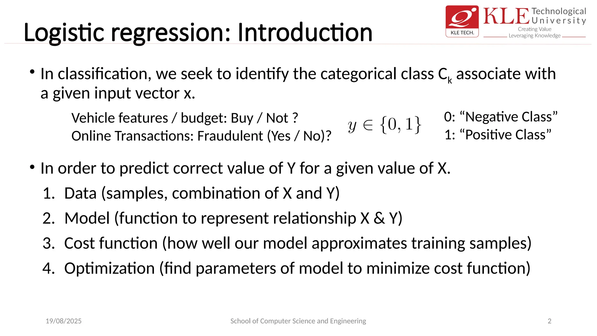
• In classification, we seek to identify the categorical class Ck associate with
a given input vector x.
• In order to predict correct value of Y for a given value of X.
1. Data (samples, combination of X and Y)
2. Model (function to represent relationship X & Y)
3. Cost function (how well our model approximates training samples)
4. Optimization (find parameters of model to minimize cost function)
19/08/2025 School of Computer Science and Engineering 2
Vehicle features / budget: Buy / Not ?
Online Transactions: Fraudulent (Yes / No)?
0: “Negative Class”
1: “Positive Class”

3. Logistic regression- data
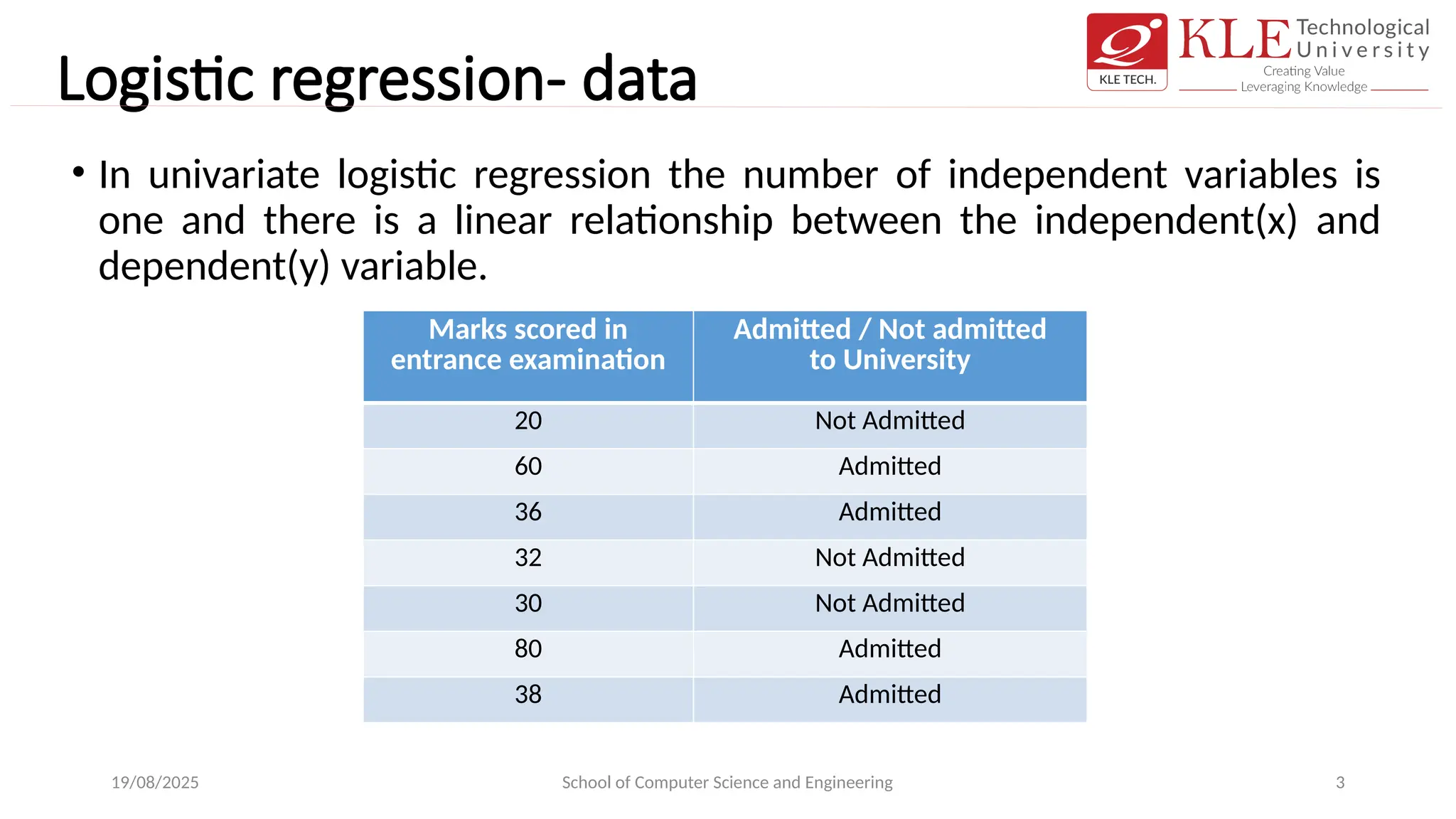
• In univariate logistic regression the number of independent variables is
one and there is a linear relationship between the independent(x) and
dependent(y) variable.
19/08/2025 School of Computer Science and Engineering 3
Marks scored in
entrance examination
Admitted / Not admitted
to University
20 Not Admitted
60 Admitted
36 Admitted
32 Not Admitted
30 Not Admitted
80 Admitted
38 Admitted

4. Logistic regression: Hypothesis
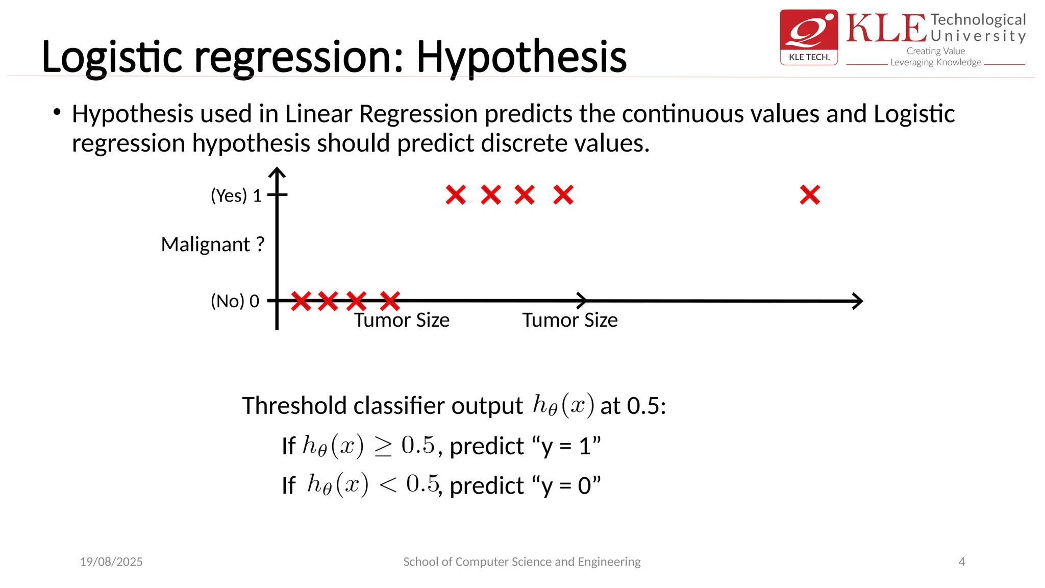
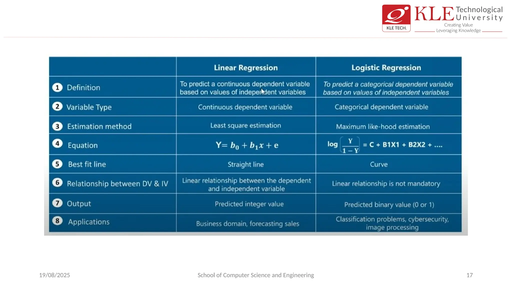
• Hypothesis used in Linear Regression predicts the continuous values and Logistic
regression hypothesis should predict discrete values.
19/08/2025 School of Computer Science and Engineering 4
Tumor Size
Threshold classifier output at 0.5:
If , predict “y = 1”
If , predict “y = 0”
Tumor Size
Malignant ?
(Yes) 1
(No) 0

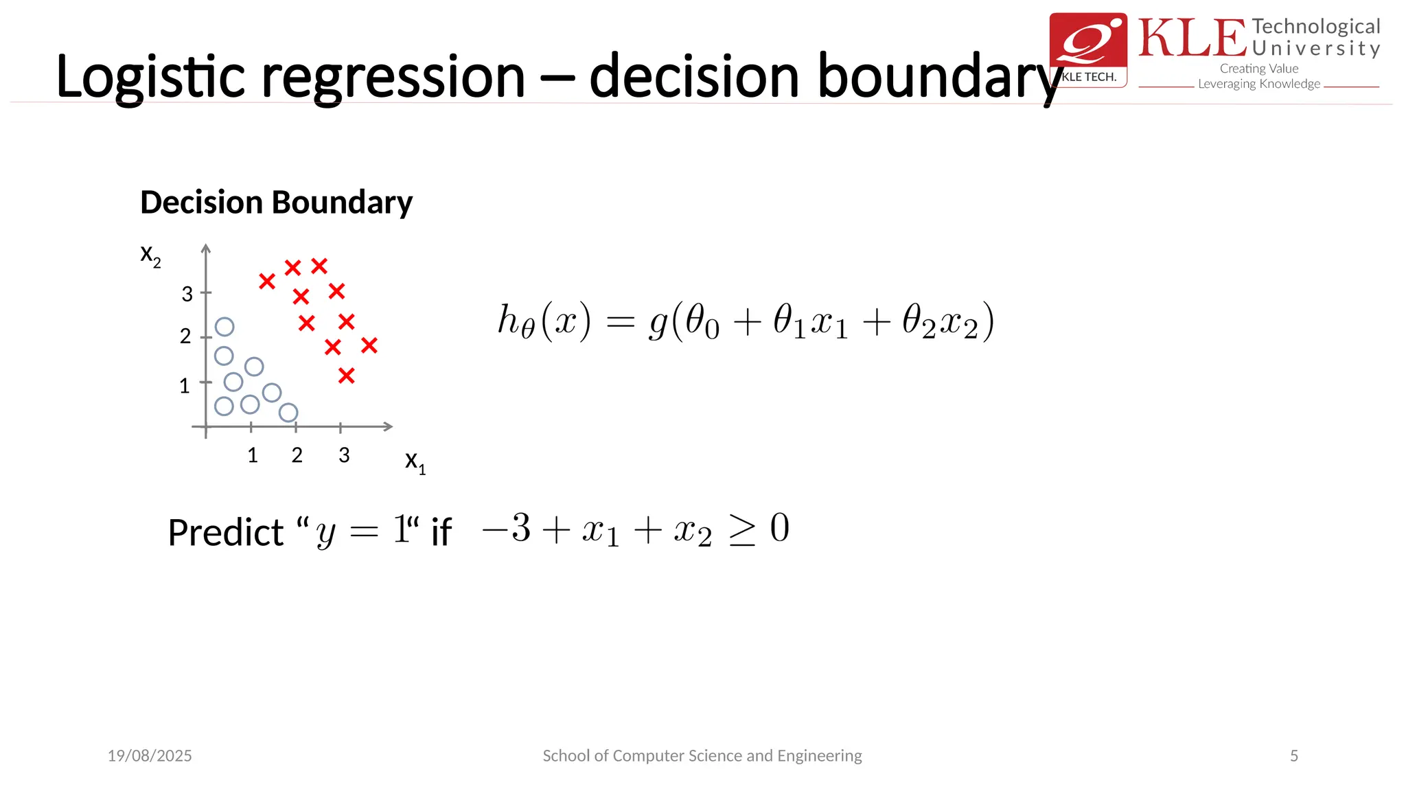
5. Logistic regression – decision boundary
19/08/2025 School of Computer Science and Engineering 5
x1
x2
Decision Boundary
1 2 3
1
2
3
Predict “ “ if

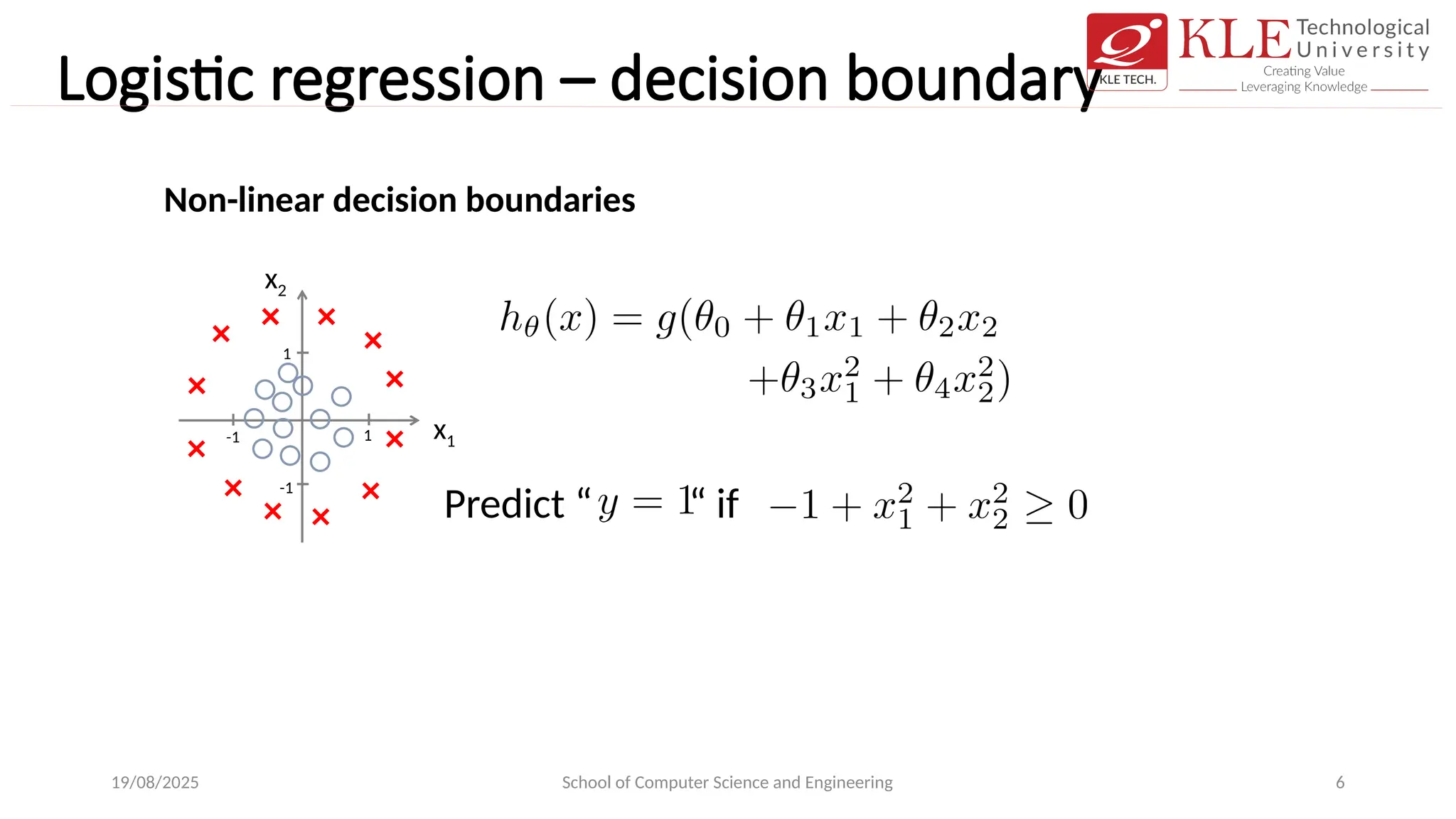
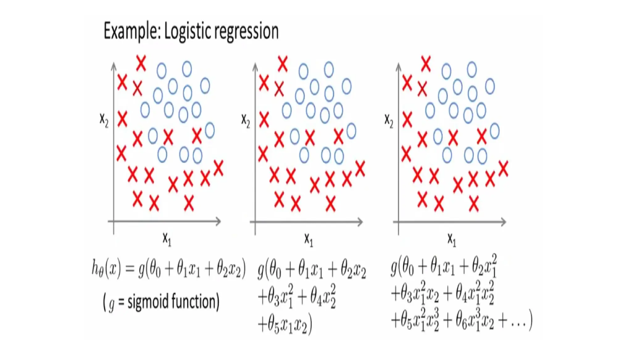
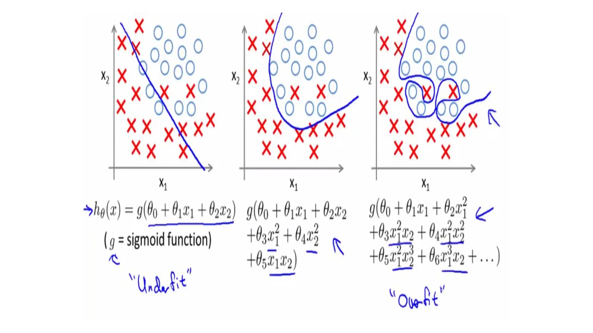
6. Logistic regression – decision boundary
19/08/2025 School of Computer Science and Engineering 6
Non-linear decision boundaries
x1
x2
Predict “ “ if
1
-1
-1
1

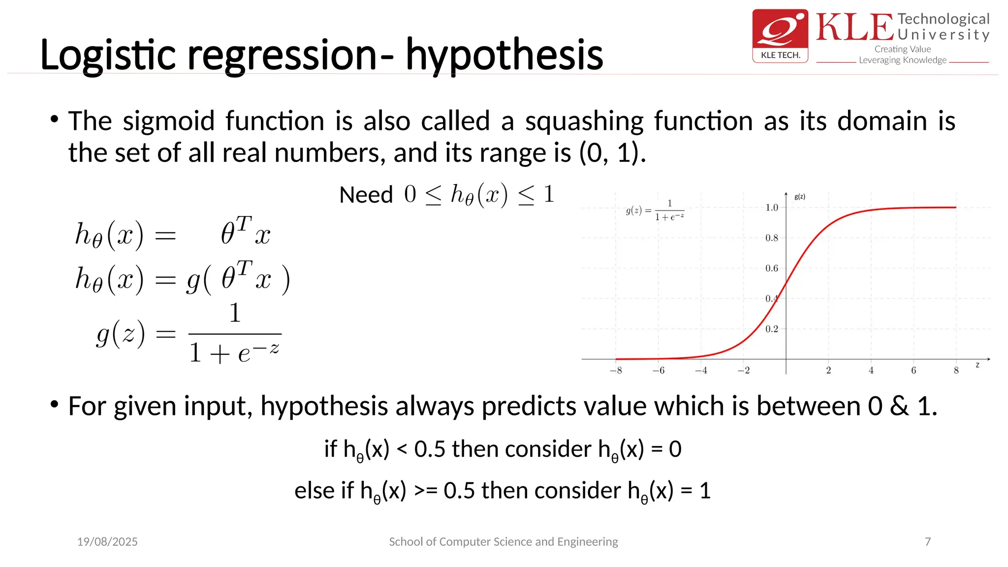
7. Logistic regression- hypothesis
• The sigmoid function is also called a squashing function as its domain is
the set of all real numbers, and its range is (0, 1).
• For given input, hypothesis always predicts value which is between 0 & 1.
if hθ(x) < 0.5 then consider hθ(x) = 0
else if hθ(x) >= 0.5 then consider hθ(x) = 1
19/08/2025 School of Computer Science and Engineering 7
Need

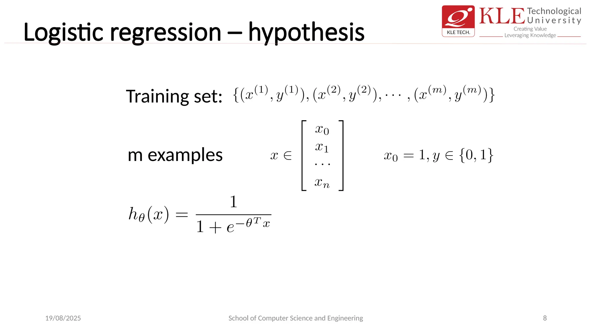
8. Logistic regression – hypothesis
19/08/2025 School of Computer Science and Engineering 8
Training set:
m examples

9. Logistic regression- hypothesis
19/08/2025 School of Computer Science and Engineering 9
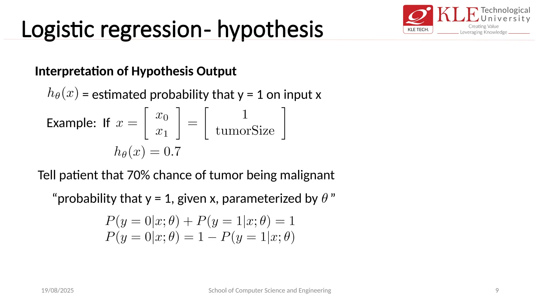
Interpretation of Hypothesis Output
= estimated probability that y = 1 on input x
Tell patient that 70% chance of tumor being malignant
Example: If
“probability that y = 1, given x, parameterized by ”

10. Logistic regression – cost function
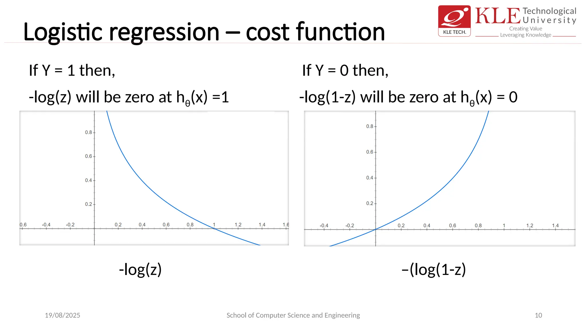
If Y = 1 then, If Y = 0 then,
-log(z) will be zero at hθ(x) =1 -log(1-z) will be zero at hθ(x) = 0
-log(z) –(log(1-z)
19/08/2025 School of Computer Science and Engineering 10

11. Logistic regression – cost function
19/08/2025 School of Computer Science and Engineering 11
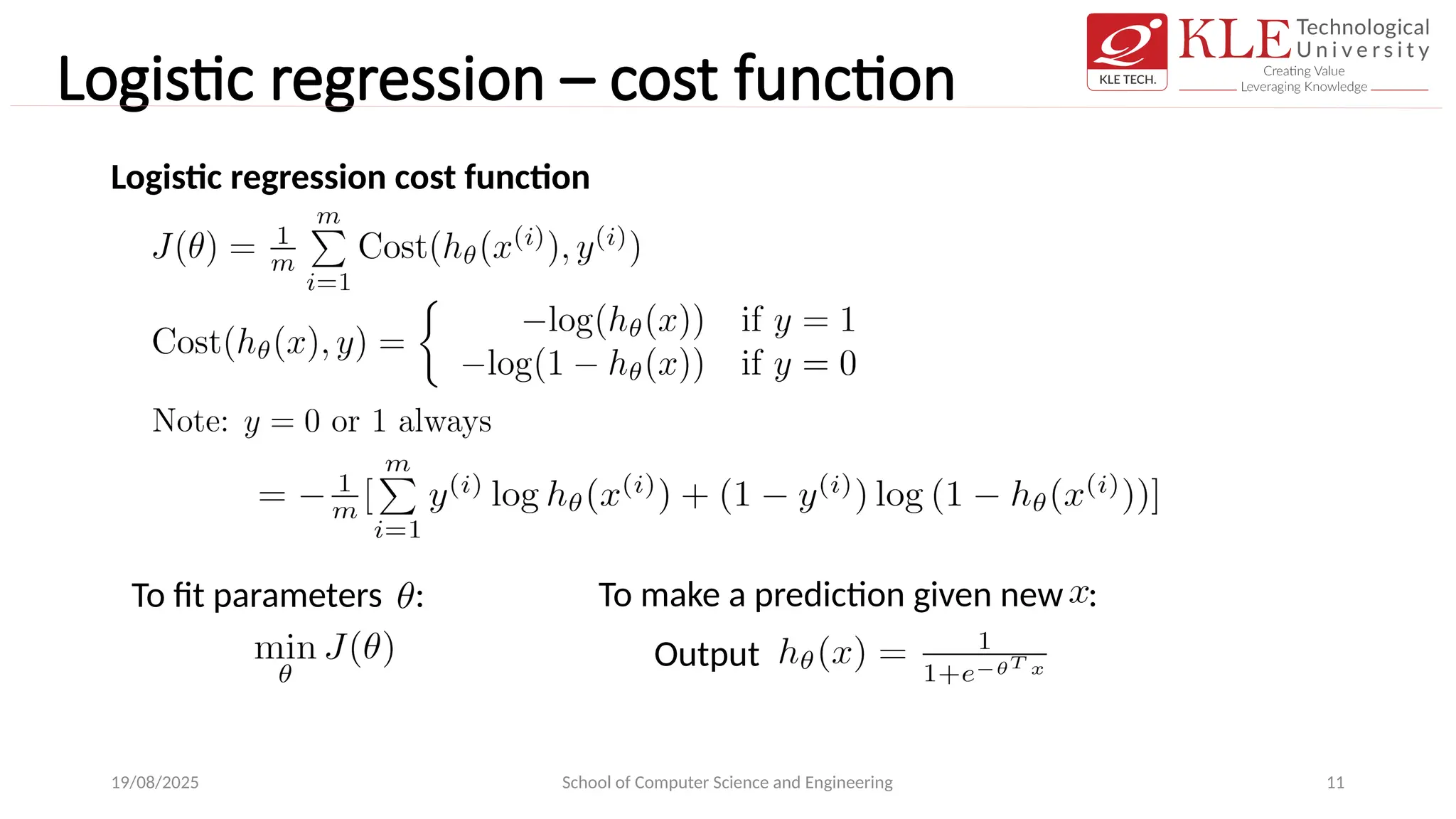
Logistic regression cost function
Output
To fit parameters : To make a prediction given new :

12. Logistic regression- optimization
19/08/2025 School of Computer Science and Engineering 12
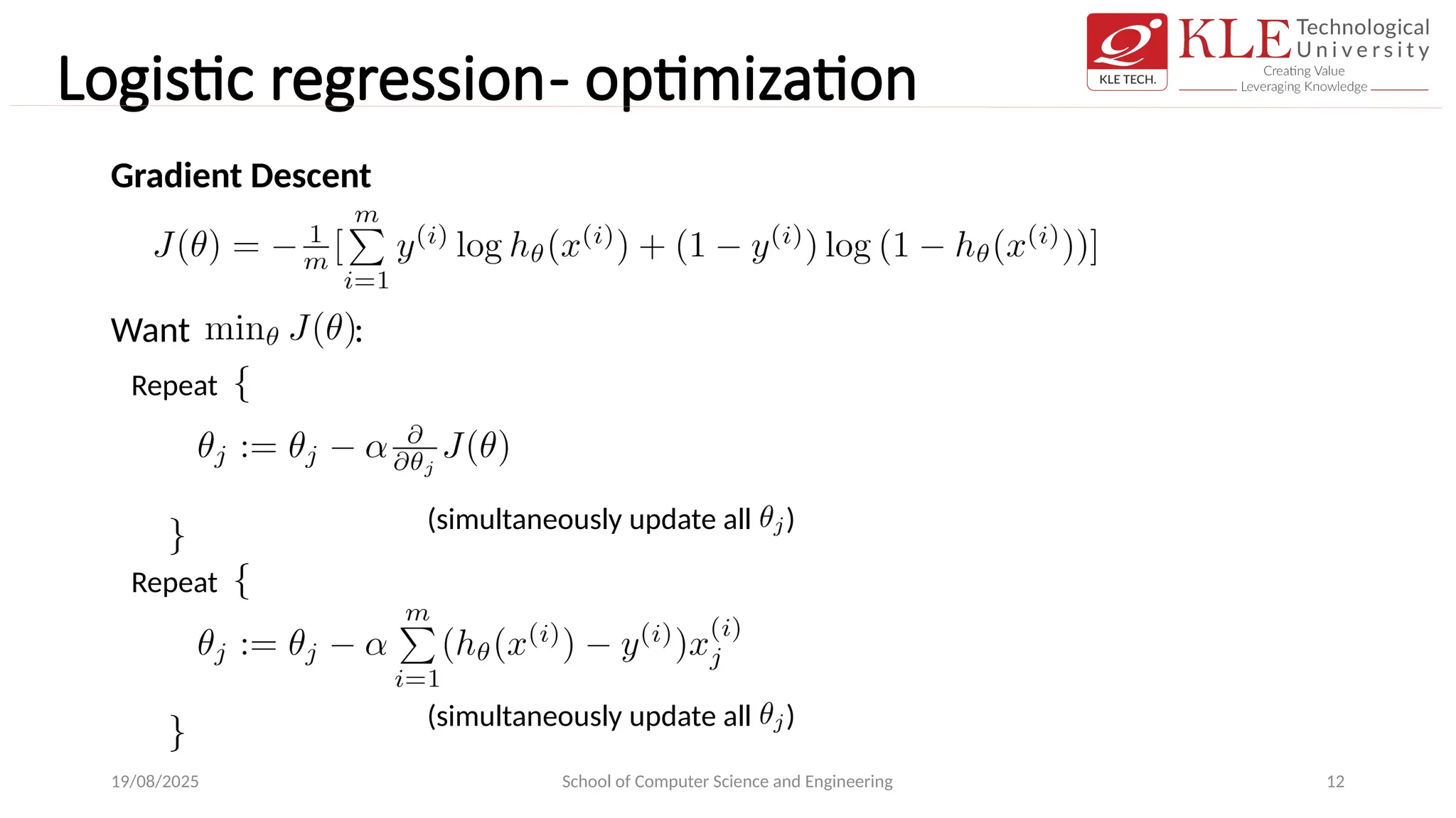
Gradient Descent
Want :
Repeat
(simultaneously update all )
(simultaneously update all )
Repeat

13. Logistic regression – multiclass
19/08/2025 School of Computer Science and Engineering 13
Email foldering/tagging: Work, Friends, Family, Hobby
Medical diagrams: Not ill, Cold, Flu
Weather: Sunny, Cloudy, Rain, Snow

14. Logistic regression – multiclass
19/08/2025 School of Computer Science and Engineering 14
x1
x2
x1
x2
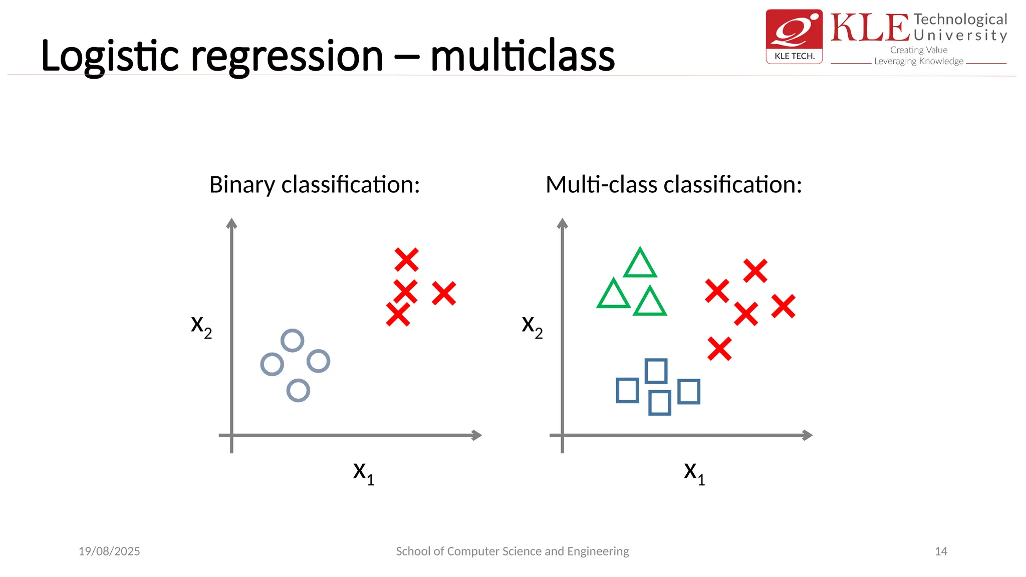
Binary classification: Multi-class classification:

15. Logistic regression – multiclass
19/08/2025 School of Computer Science and Engineering 15
x1
x2
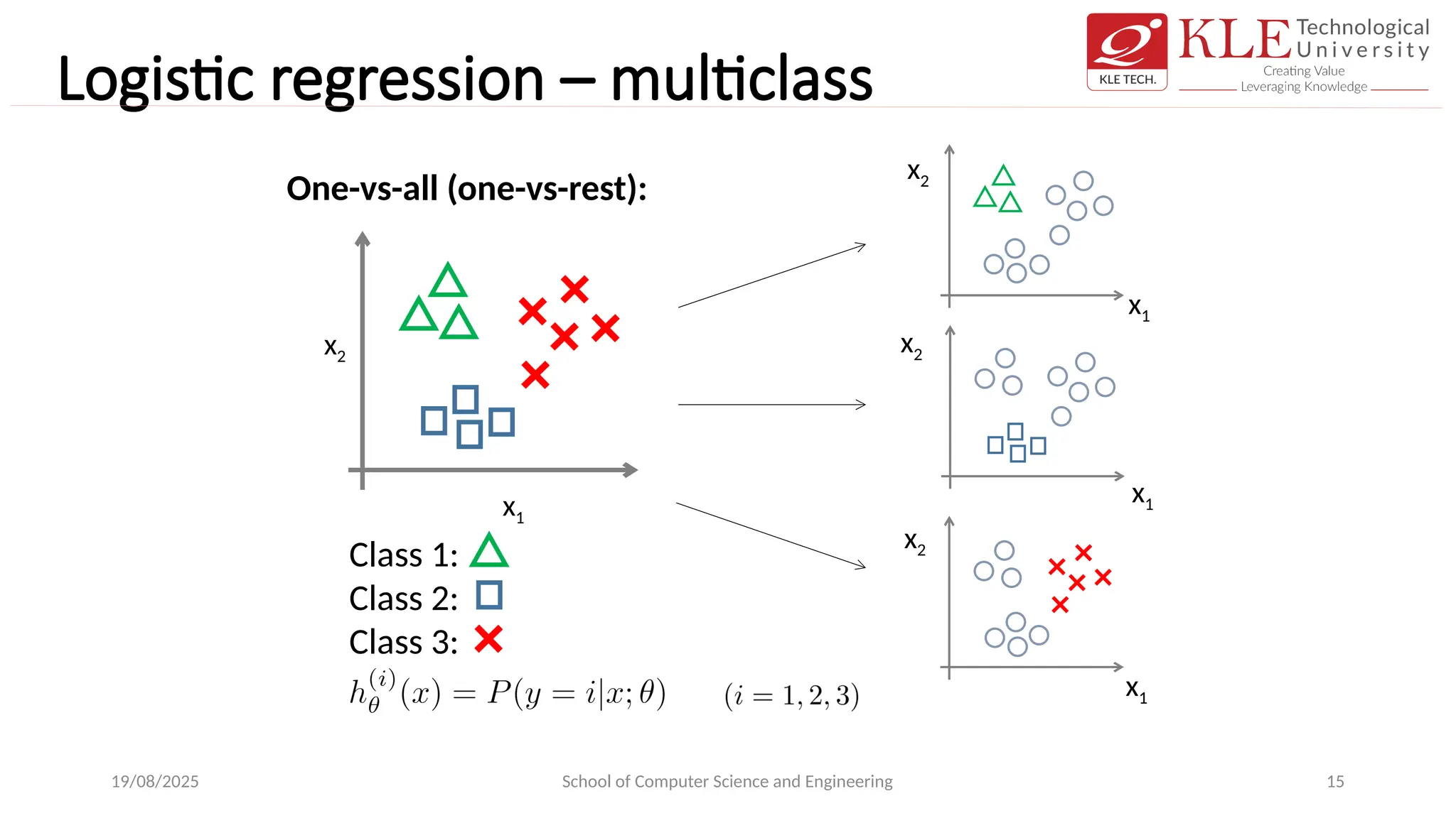
One-vs-all (one-vs-rest):
Class 1:
Class 2:
Class 3:
x1
x2
x1
x2
x1
x2

16. Logistic regression – multiclass
19/08/2025 School of Computer Science and Engineering 16
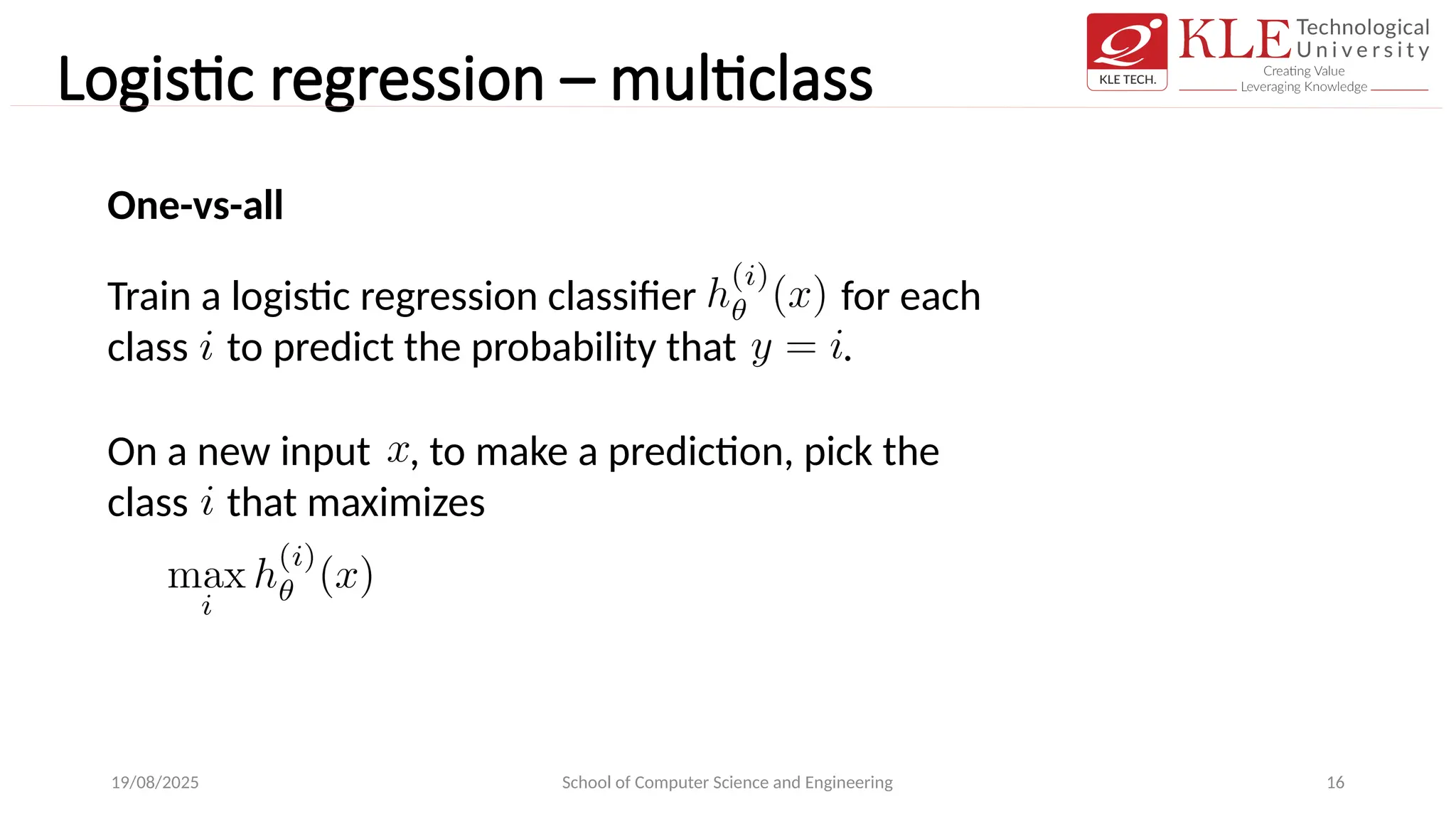
One-vs-all
Train a logistic regression classifier for each
class to predict the probability that .
On a new input , to make a prediction, pick the
class that maximizes

17. 19/08/2025 School of Computer Science and Engineering 17

18. Supervised Learning:
Regularization

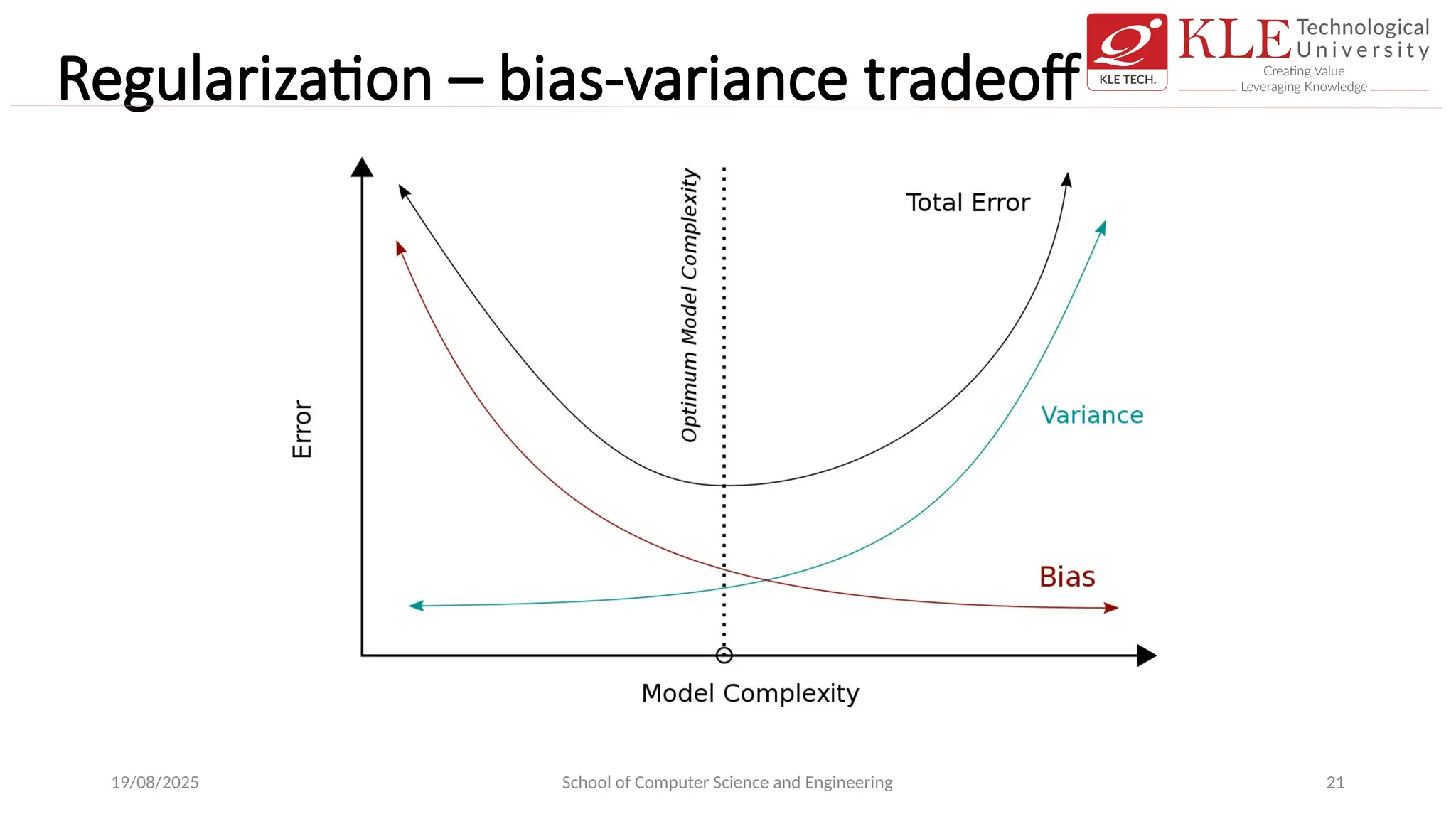
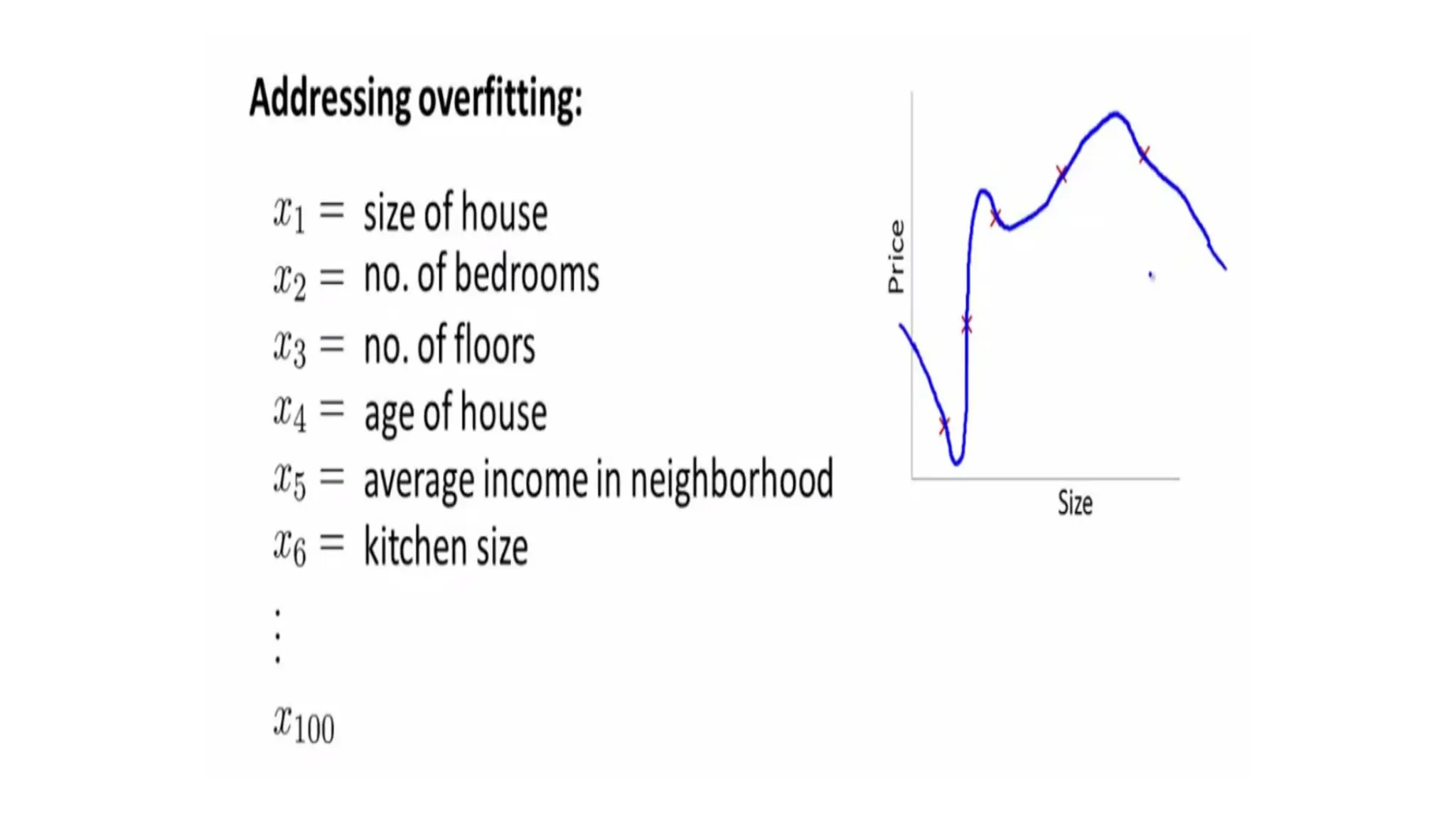
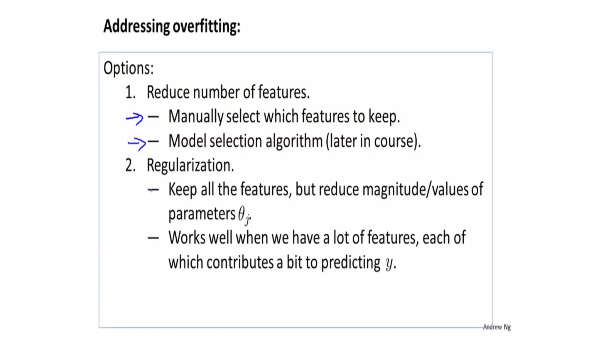
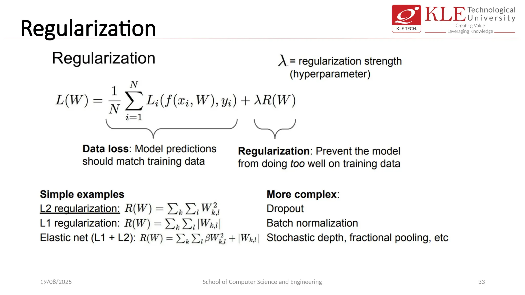
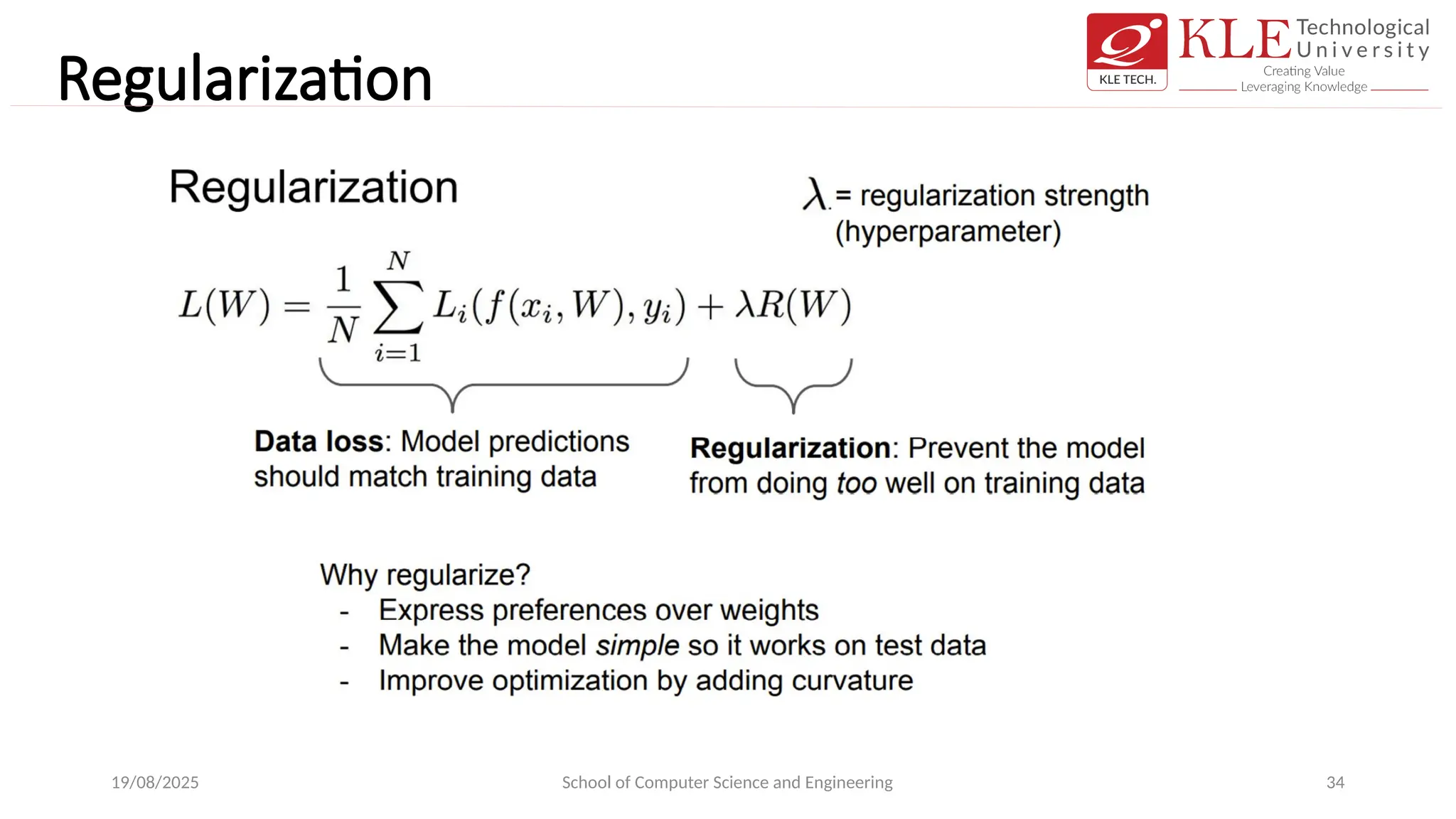
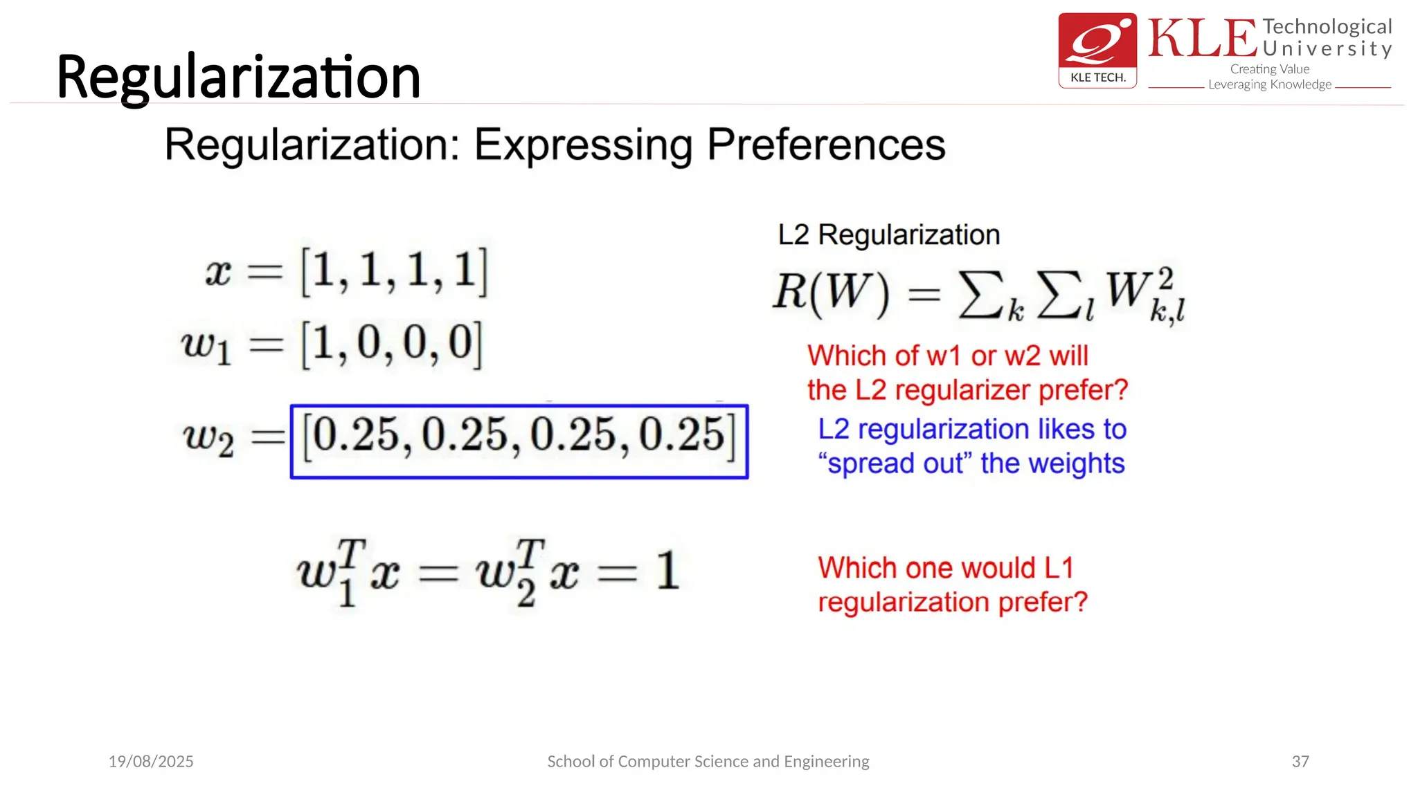
19. Regularization
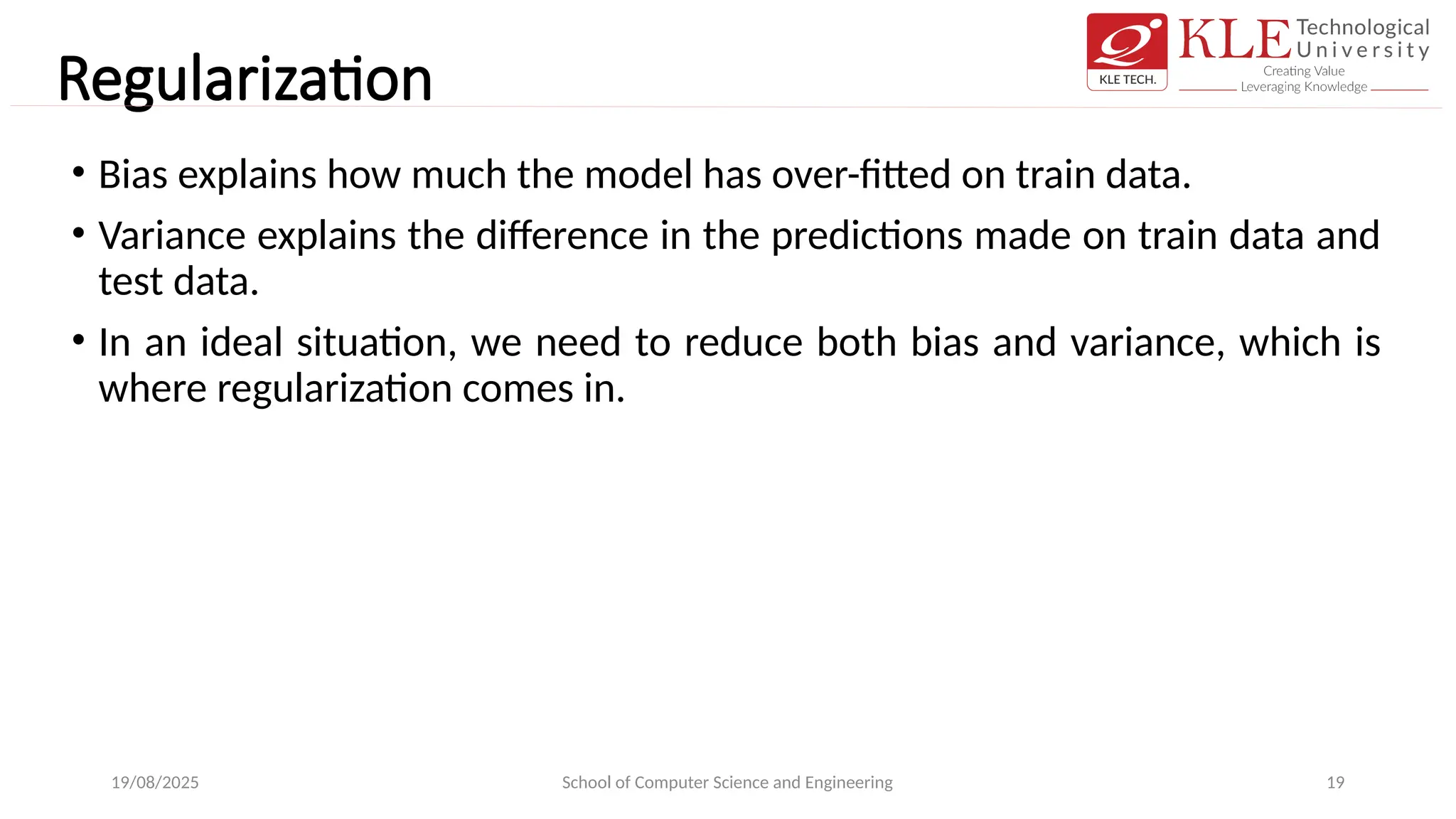
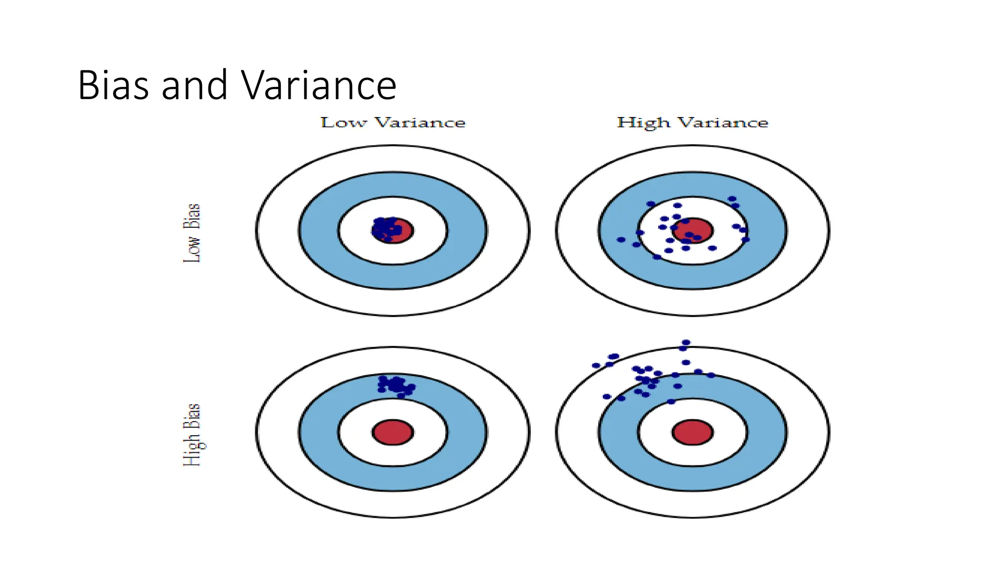
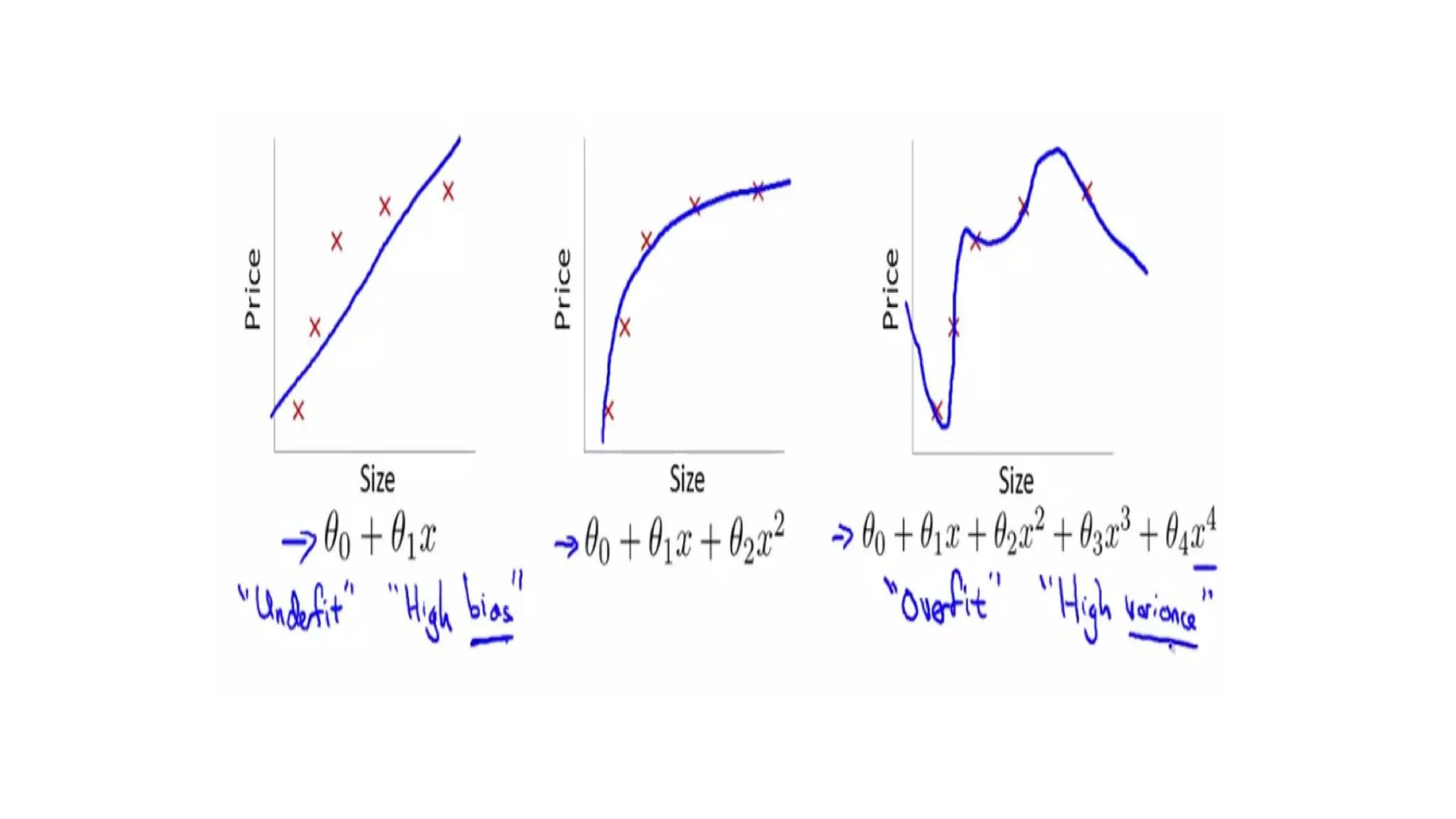
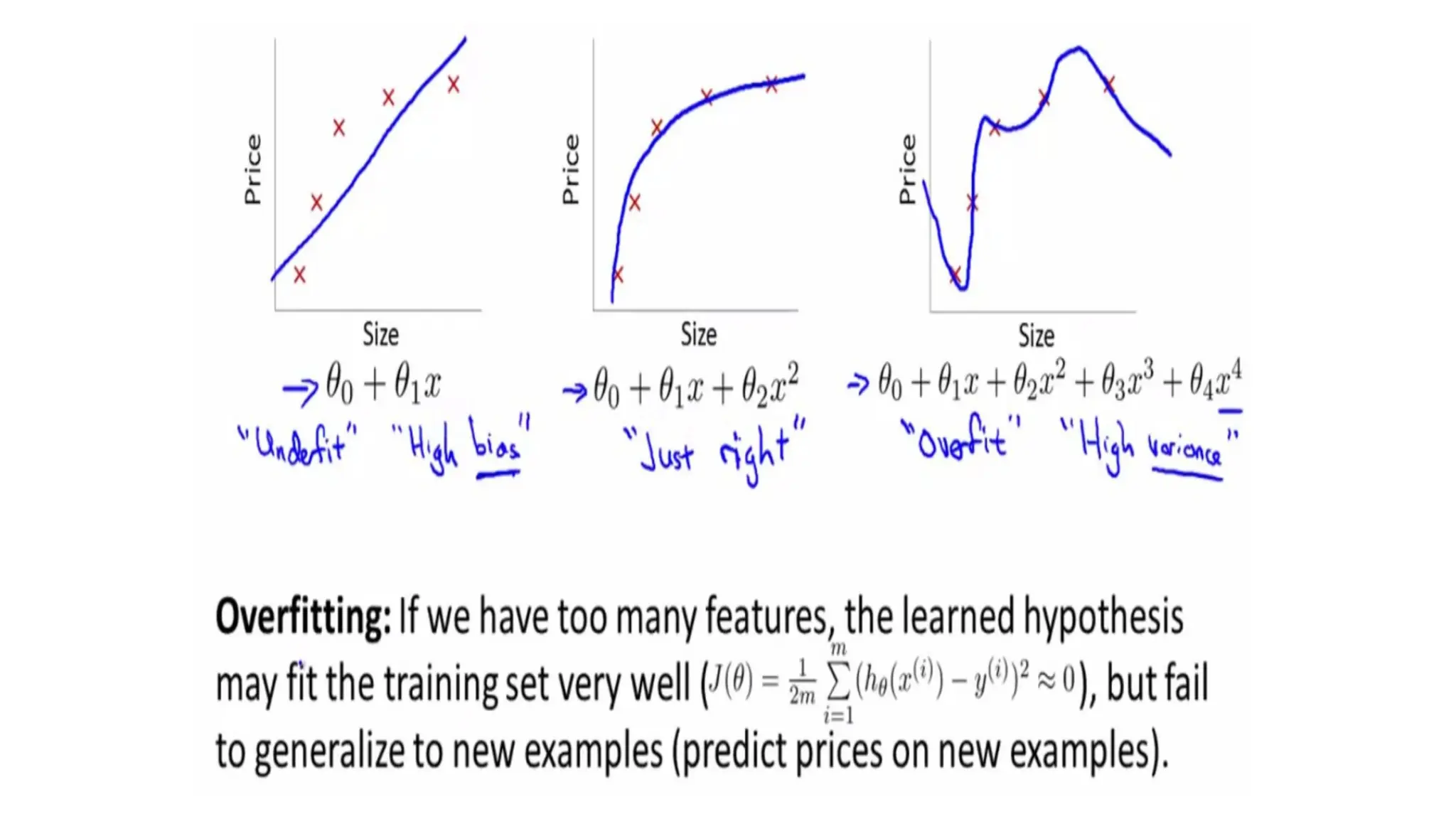
• Bias explains how much the model has over-fitted on train data.
• Variance explains the difference in the predictions made on train data and
test data.
• In an ideal situation, we need to reduce both bias and variance, which is
where regularization comes in.
19/08/2025 School of Computer Science and Engineering 19

20. Bias and Variance

21. Regularization – bias-variance tradeoff
19/08/2025 School of Computer Science and Engineering 21

31. Regularization
19/08/2025 School of Computer Science and Engineering 31

32. Regularization
19/08/2025 School of Computer Science and Engineering 32

33. Regularization
19/08/2025 School of Computer Science and Engineering 33

34. Regularization
19/08/2025 School of Computer Science and Engineering 34

35. Regularization
19/08/2025 School of Computer Science and Engineering 35

36. Regularization
19/08/2025 School of Computer Science and Engineering 36

37. Regularization
19/08/2025 School of Computer Science and Engineering 37

38. Regularization
19/08/2025 School of Computer Science and Engineering 38

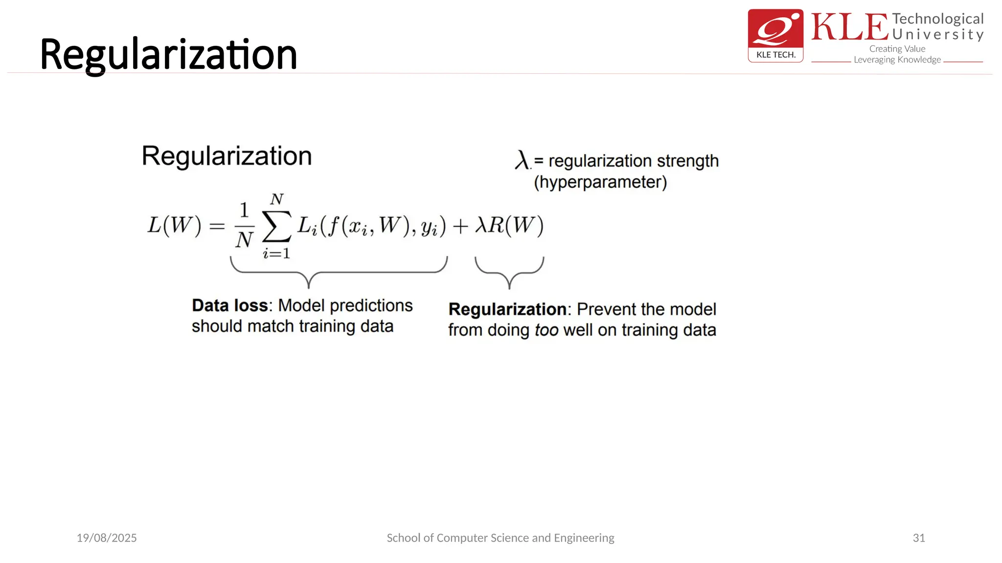
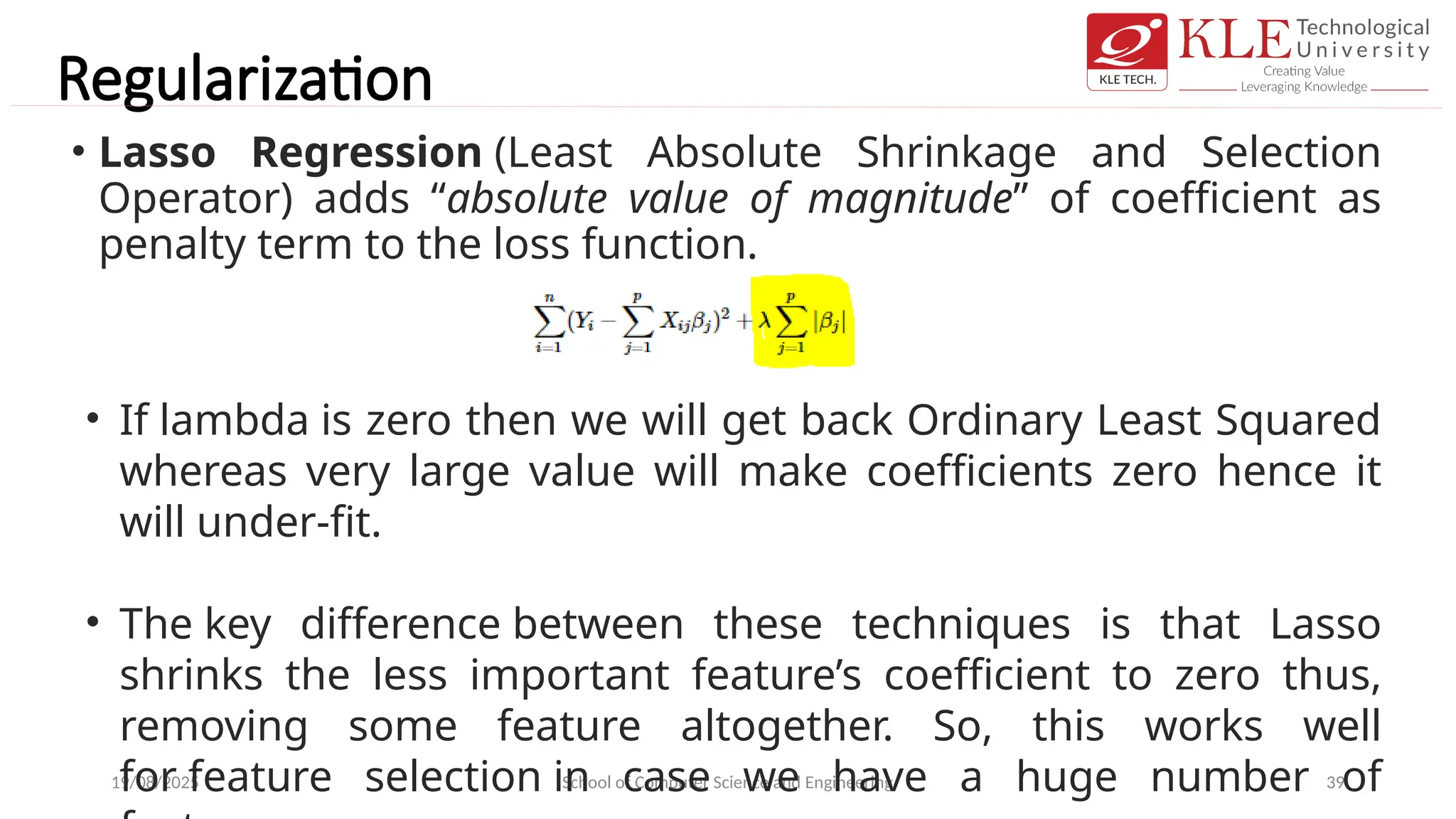
39. Regularization
• Lasso Regression (Least Absolute Shrinkage and Selection
Operator) adds “absolute value of magnitude” of coefficient as
penalty term to the loss function.
19/08/2025 School of Computer Science and Engineering 39
• If lambda is zero then we will get back Ordinary Least Squared
whereas very large value will make coefficients zero hence it
will under-fit.
• The key difference between these techniques is that Lasso
shrinks the less important feature’s coefficient to zero thus,
removing some feature altogether. So, this works well
for feature selection in case we have a huge number of

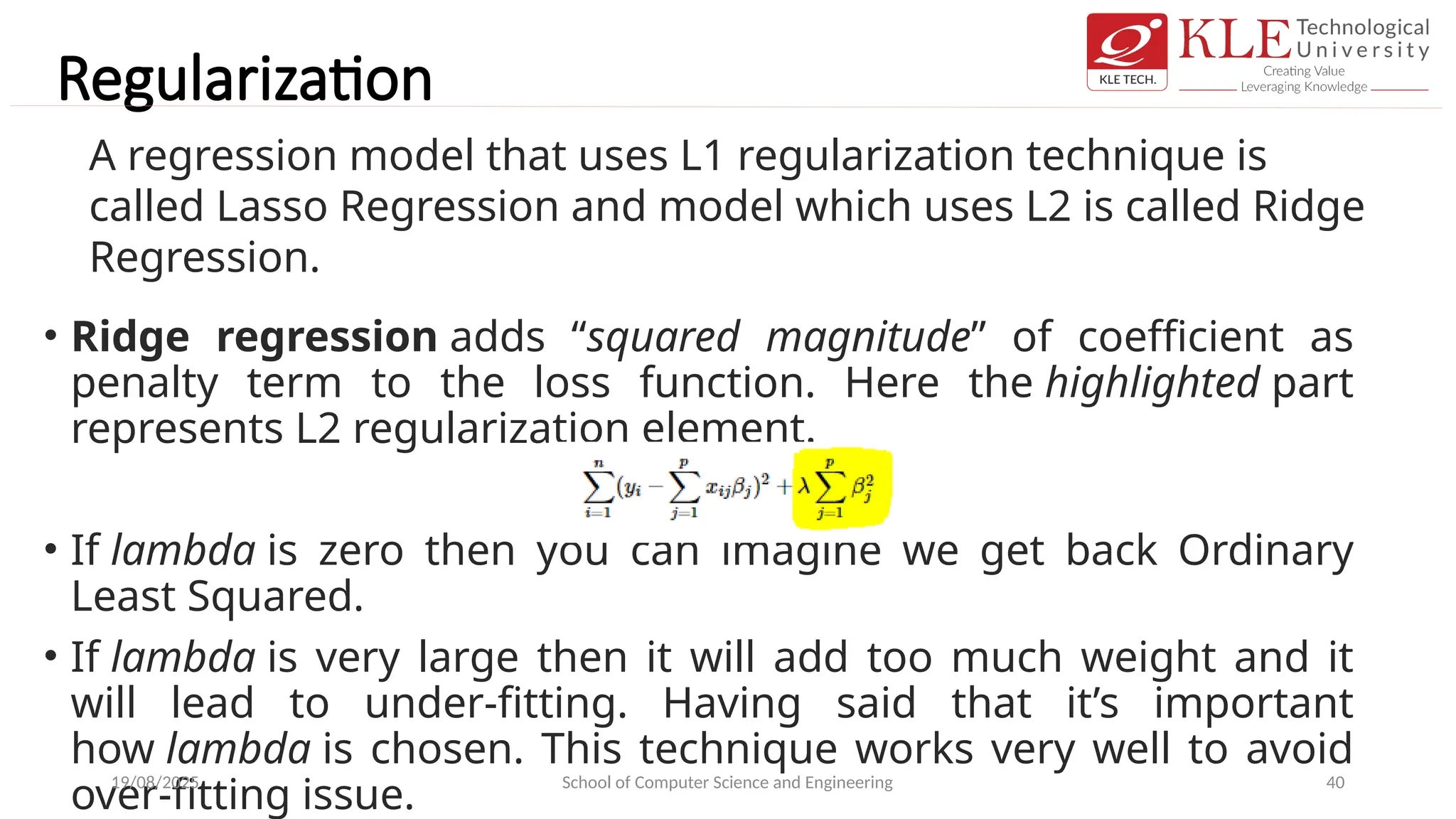
40. Regularization
• Ridge regression adds “squared magnitude” of coefficient as
penalty term to the loss function. Here the highlighted part
represents L2 regularization element.
• If lambda is zero then you can imagine we get back Ordinary
Least Squared.
• If lambda is very large then it will add too much weight and it
will lead to under-fitting. Having said that it’s important
how lambda is chosen. This technique works very well to avoid
over-fitting issue.
19/08/2025 School of Computer Science and Engineering 40
A regression model that uses L1 regularization technique is
called Lasso Regression and model which uses L2 is called Ridge
Regression.

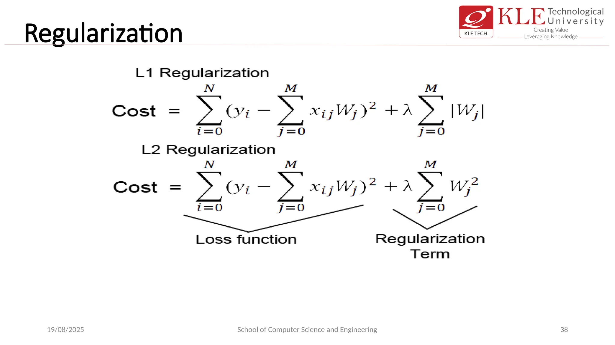
41. • we can see from the formula of L1 and L2 regularization, L1
regularization adds the penalty term in cost function by
adding the absolute value of weight(Wj) parameters, while L2
regularization adds the squared value of weights(Wj) in the
cost function.
• L1 regularization helps in feature selection by eliminating the
features that are not important. This is helpful when the
number of feature points are large in number.
• L1 regularization it will estimate around the median of the
data.
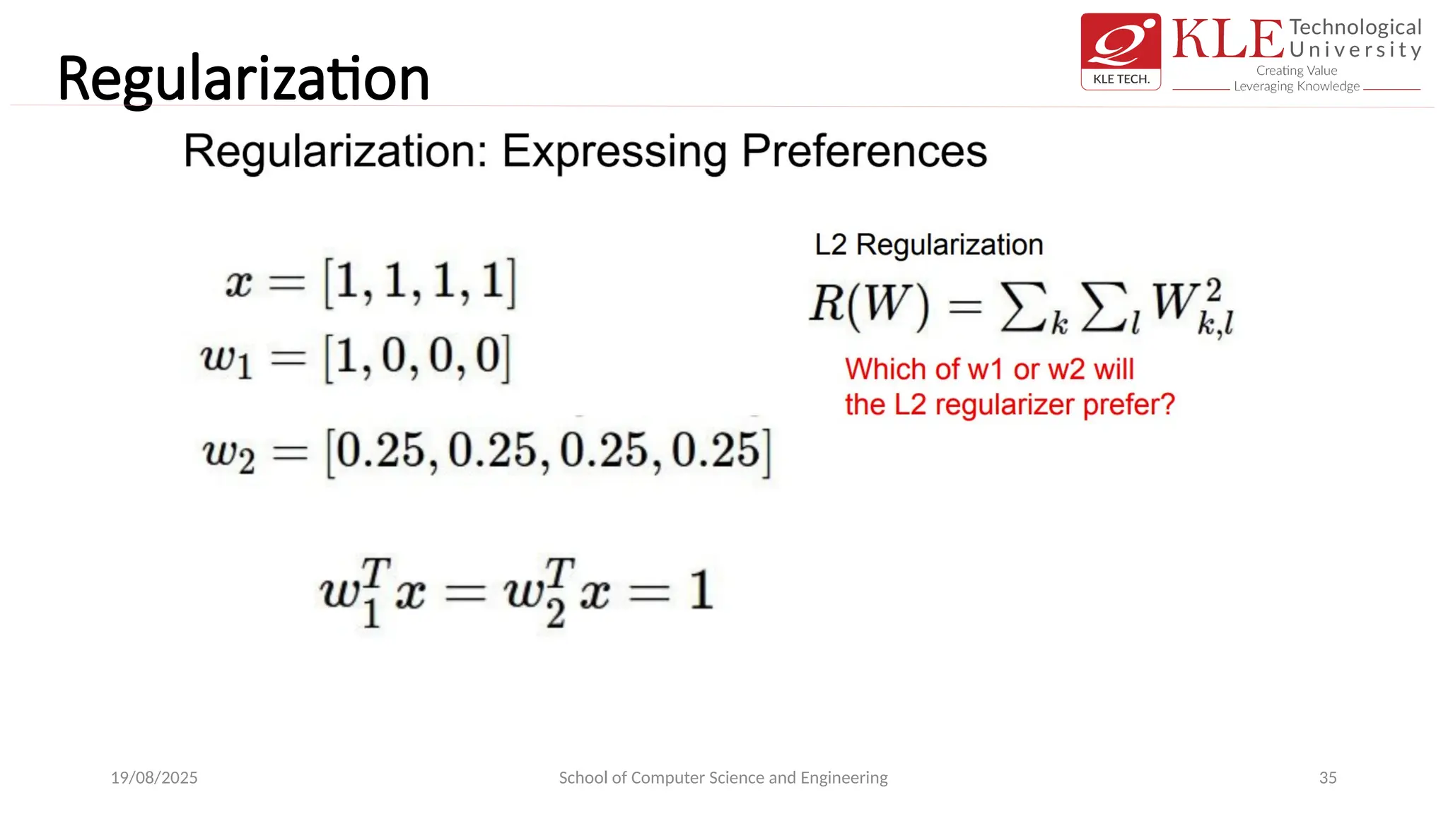
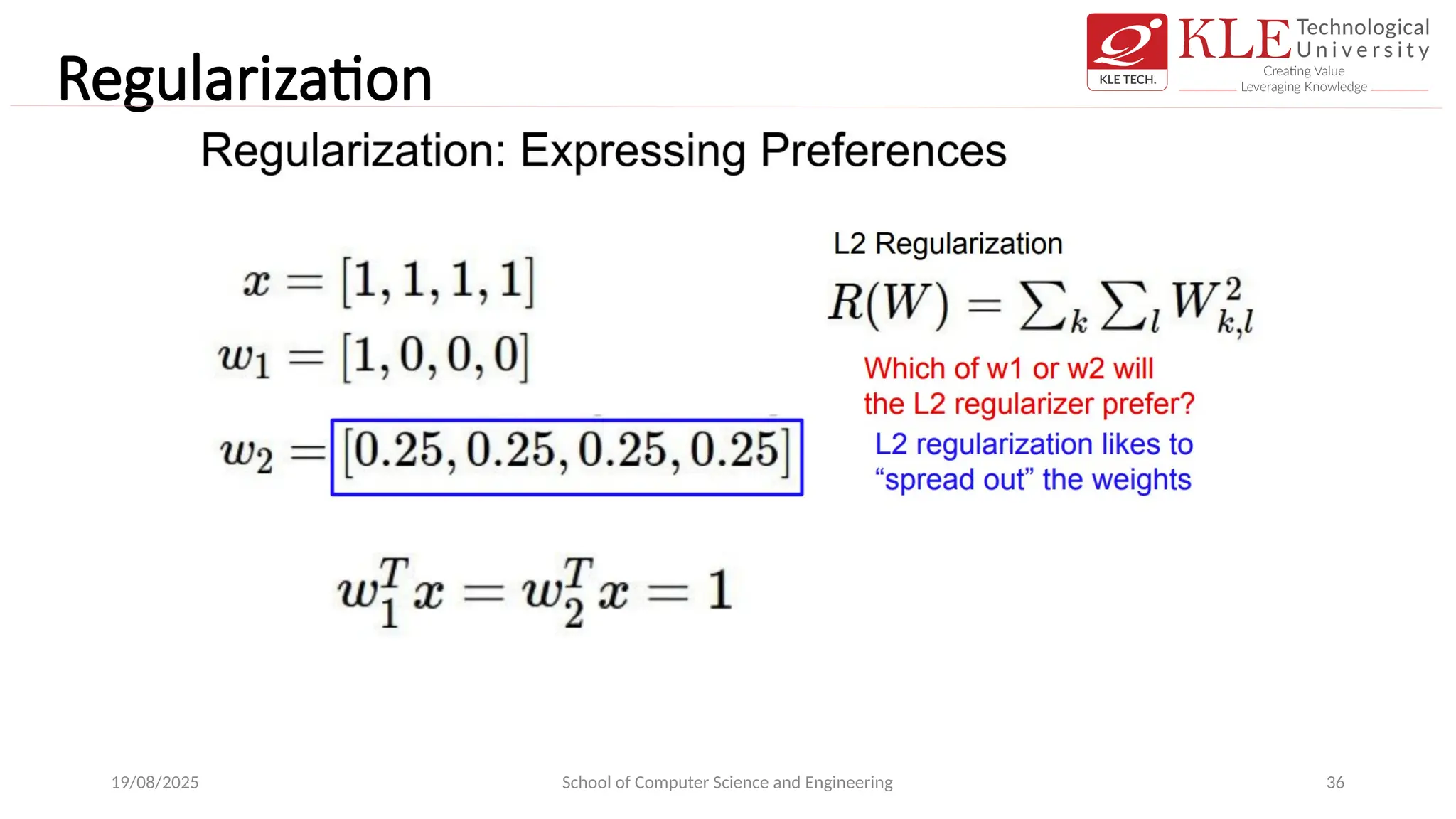
• L2 regularization, while calculating the loss function in the
gradient calculation step, the loss function tries to minimize
the loss by subtracting it from the average of the data
19/08/2025 School of Computer Science and Engineering 41

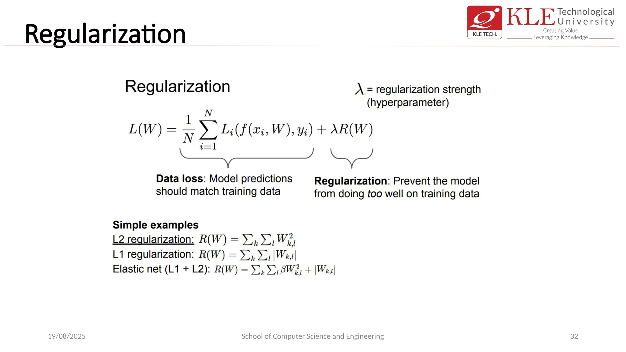
42. Regularization
• L1 Regularization aka Lasso Regularization:
• This add regularization terms in the model which are function of absolute value of
the coefficients of parameters.
• The coefficient of the parameters can be driven to zero as well during the
regularization process. Hence this technique can be used for feature selection and
generating more parsimonious model.
• L2 Regularization aka Ridge Regularization:
• This add regularization terms in the model which are function of square of
coefficients of parameters. Coefficient of parameters can approach to zero but
never become zero and hence.
• Combination of the above two such as Elastic Nets:
• This add regularization terms in the model which are combination of both L1 and
L2 regularization.
19/08/2025 School of Computer Science and Engineering 42

43. Support Vector Machines

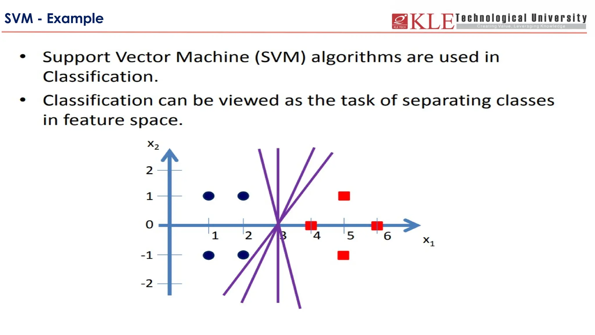
44. SVM - Introduction
-Support Vector Machine (SVM) is a supervised learning algorithm
developed by Vladimir Vapnik and it was first heard in 1992, introduced
by Vapnik, Boser and Guyon in COLT-92.
-Support Vector Machine (SVM) is a relatively simple Supervised
Machine Learning Algorithm used for classification and/or regression.
It is more preferred for classification but is sometimes very useful for
regression as well.
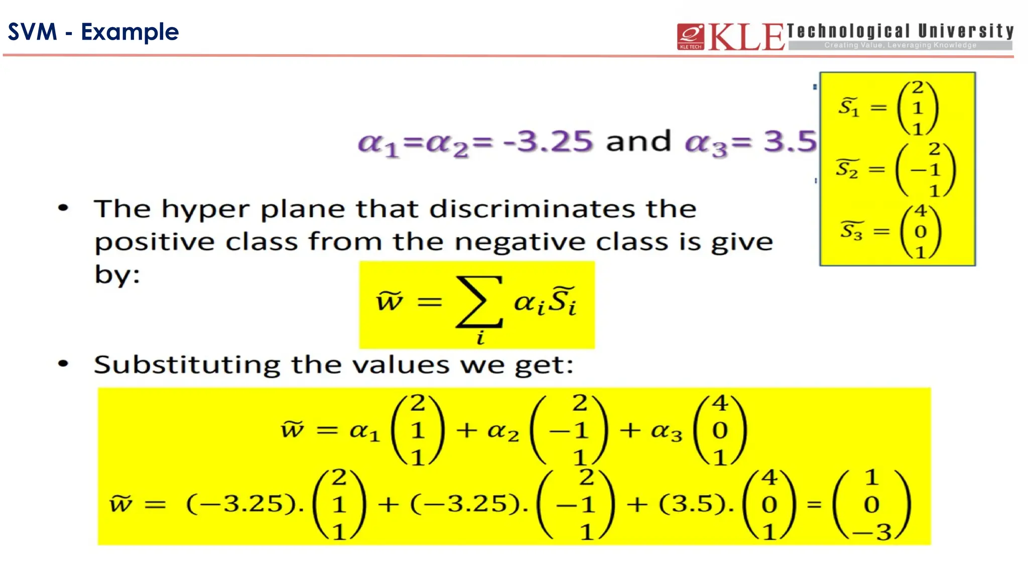
• Basically, SVM finds a hyper-plane that creates a boundary between the
types of data.
• The two results of each classifier will be :
• The data point belongs to that class OR
• The data point does not belong to that class.

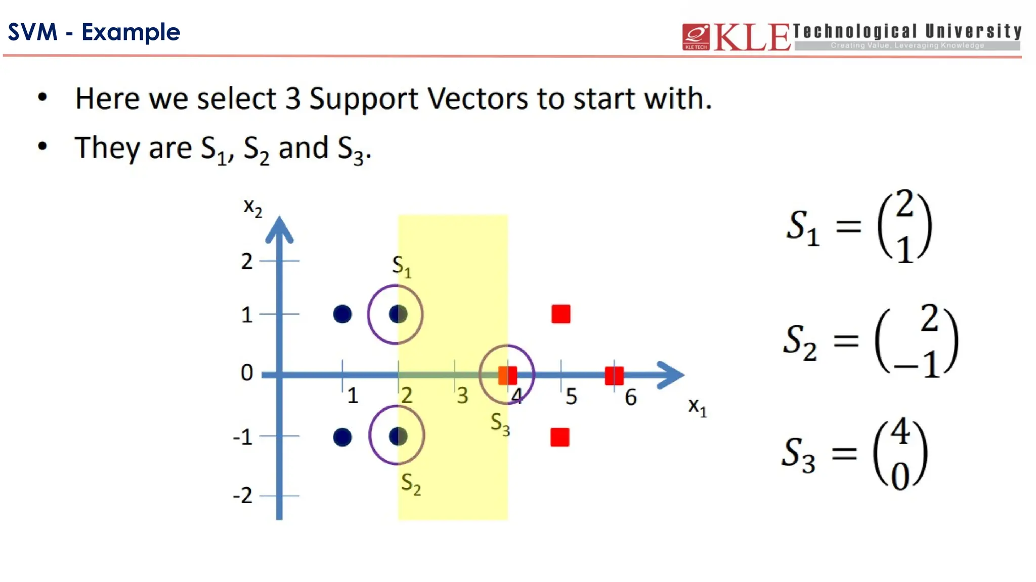
45. SVM - Introduction
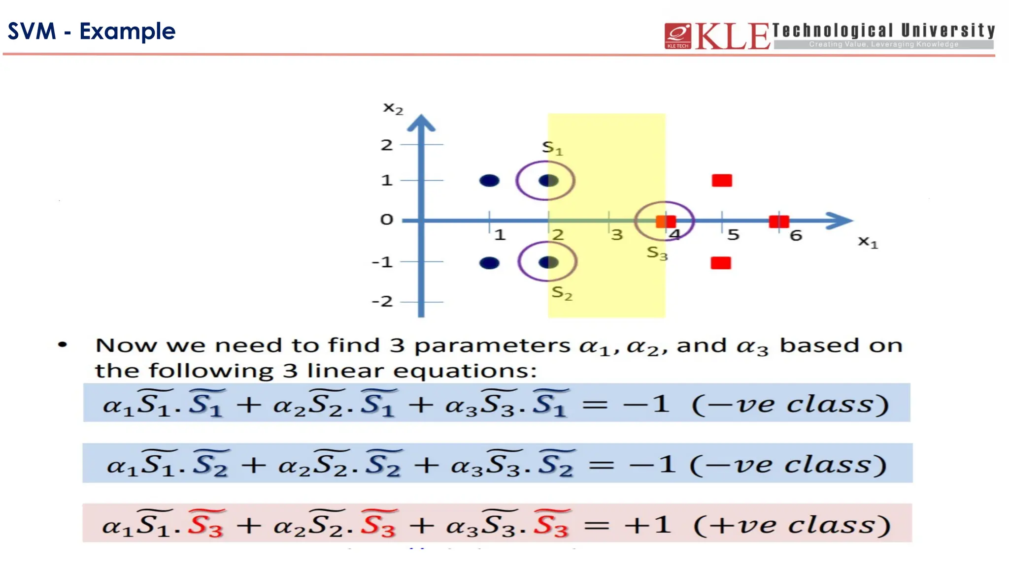
• The aim of a support vector machine algorithm is to find the best possible line,
or decision boundary, that separates the data points of different data classes.
• This boundary is called a hyperplane when working in high-dimensional feature
spaces.
• The idea is to maximize the margin, which is the distance between the hyperplane
and the closest data points of each category, thus making it easy to distinguish data
classes.
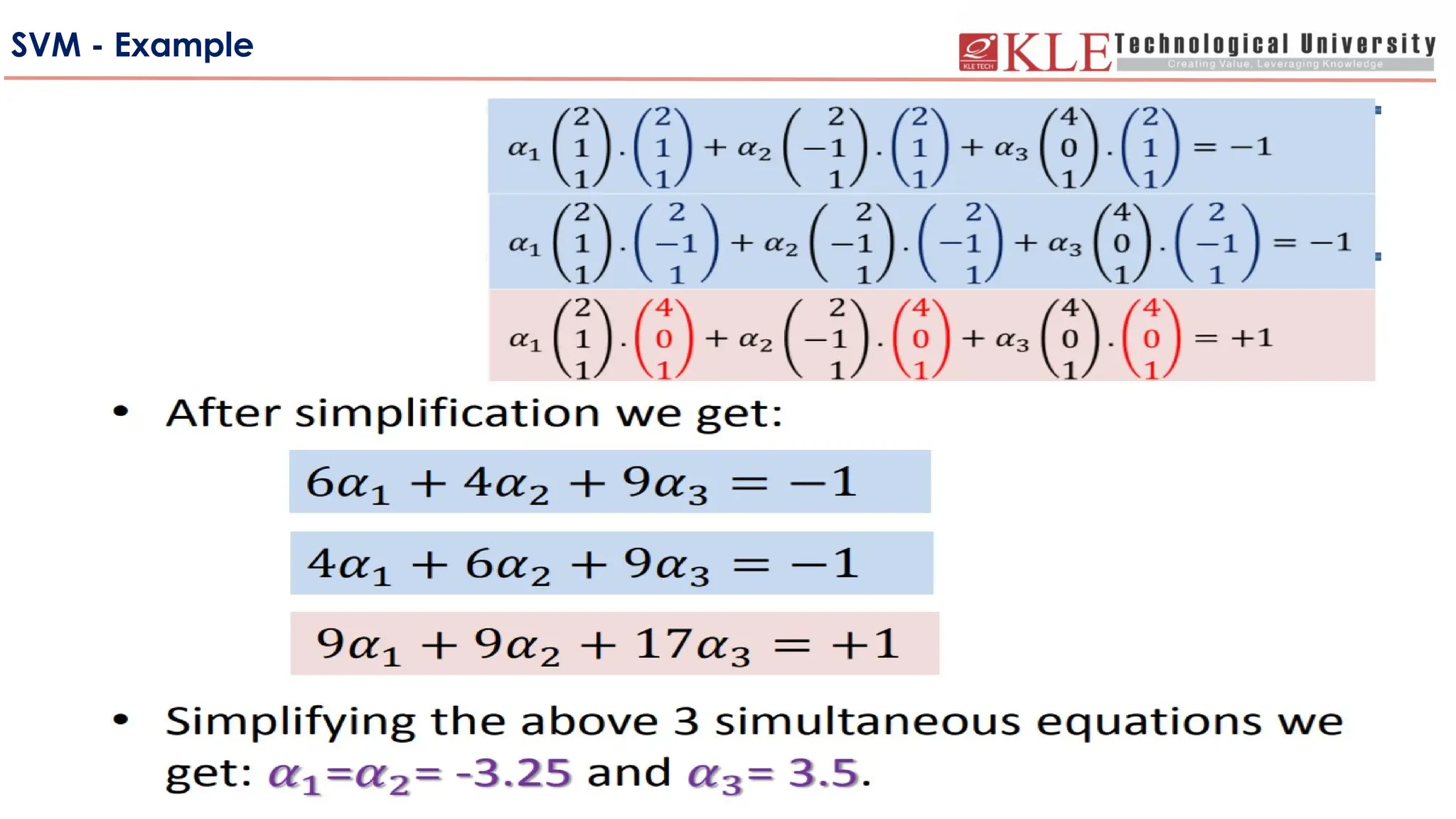
• During the training phase, SVMs use a mathematical formulation to find the
optimal hyperplane in a higher-dimensional space, often called the kernel space.
• This hyperplane is crucial because it maximizes the margin between data points of
different classes, while minimizing the classification errors.

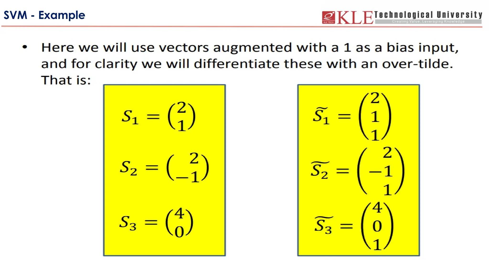
46. SVM - Introduction
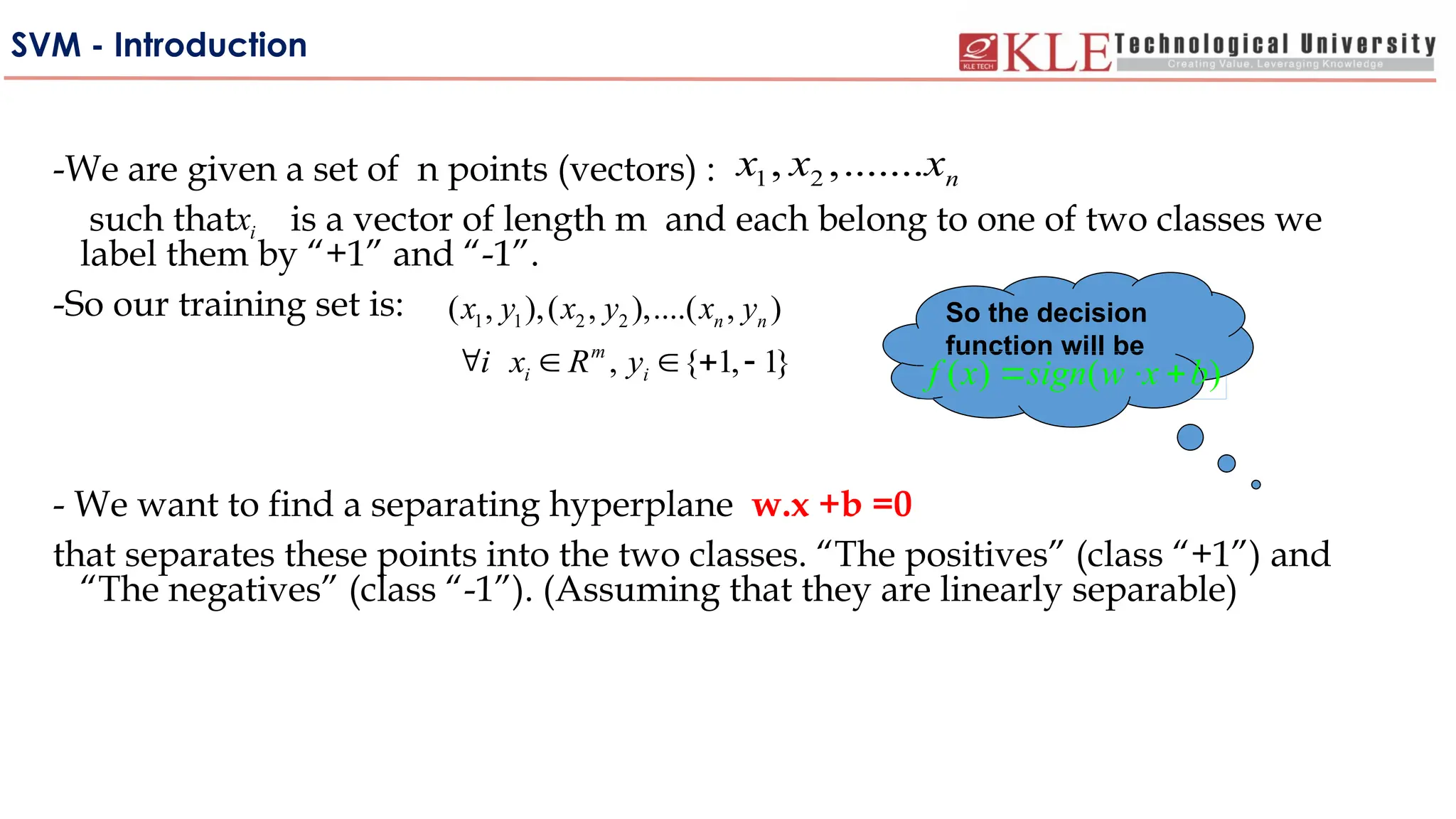
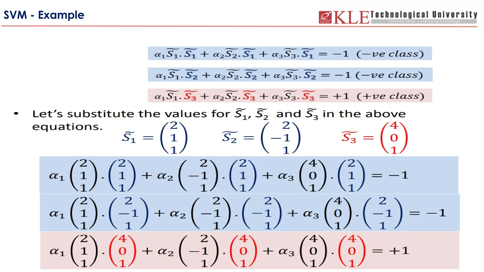
-We are given a set of n points (vectors) :
such that is a vector of length m and each belong to one of two classes we
label them by “+1” and “-1”.
-So our training set is:
- We want to find a separating hyperplane w.x +b =0
that separates these points into the two classes. “The positives” (class “+1”) and
“The negatives” (class “-1”). (Assuming that they are linearly separable)
1 2
, ,....... n
x x x
i
x
1 1 2 2
( , ),( , ),....( , )
n n
x y x y x y
, { 1, 1}
m
i i
i x R y
    
So the decision
function will be
( ) ( )
f x sign w x b
  

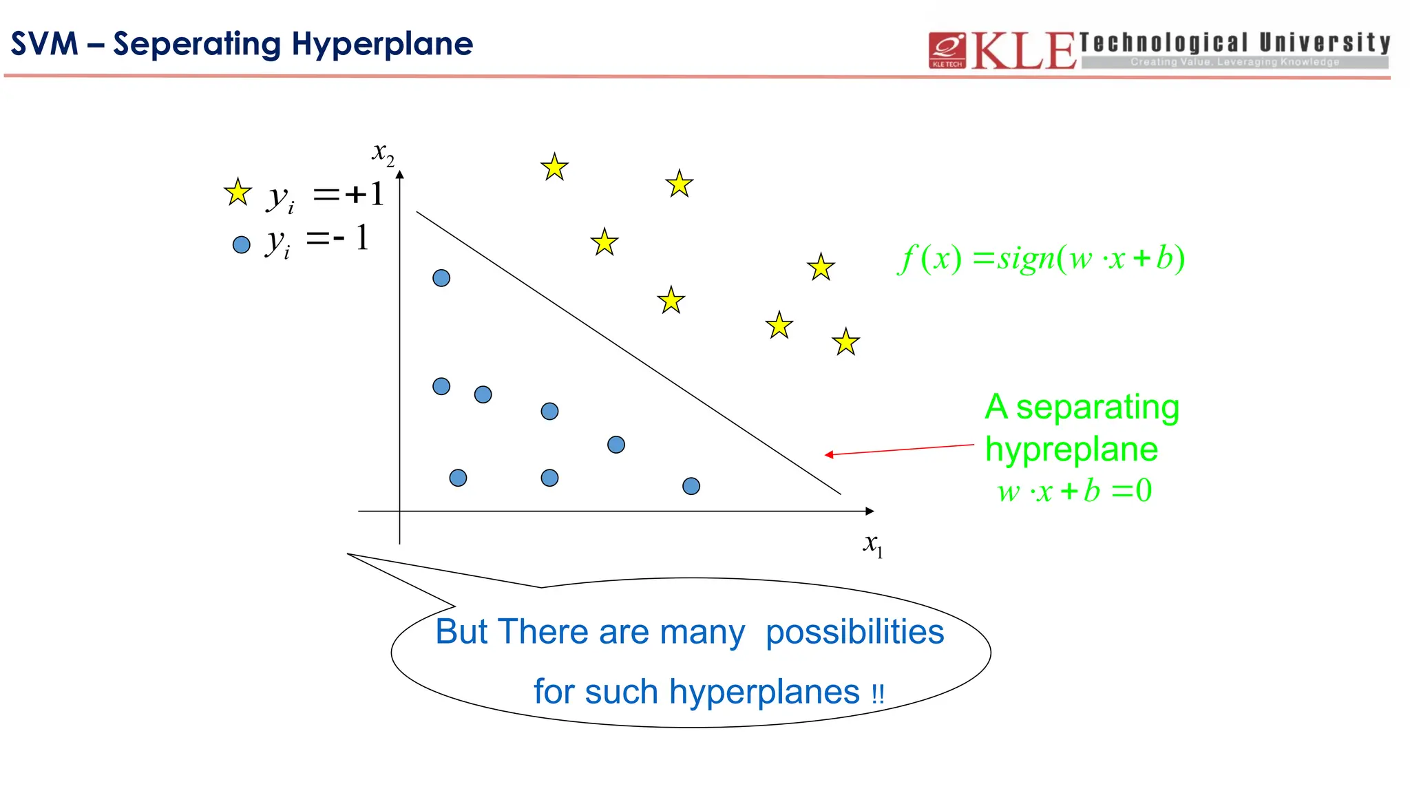
47. SVM – Seperating Hyperplane
A separating
hypreplane
1
i
y 
1
i
y 
But There are many possibilities
for such hyperplanes !!
( ) ( )
f x sign w x b
  
0
w x b
  
1
x
2
x

48. 1
i
y 
1
i
y 
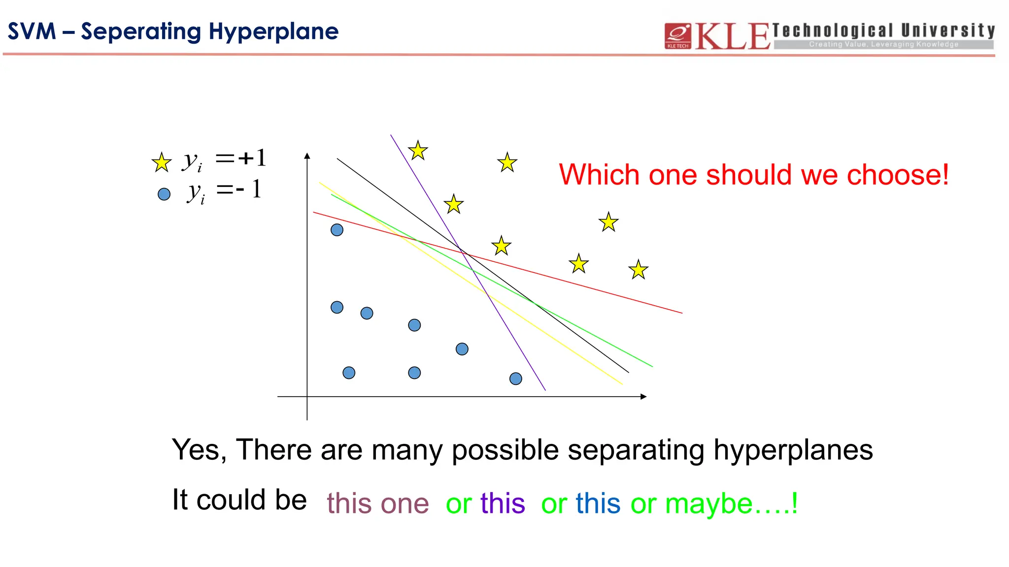
Yes, There are many possible separating hyperplanes
It could be
Which one should we choose!
this one or this or this or maybe….!
SVM – Seperating Hyperplane

49. SVM – Choosing a separating hyperplane
i
x
'
x
( )
f x
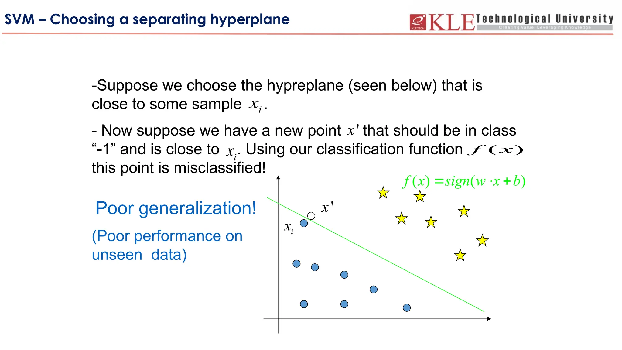
-Suppose we choose the hypreplane (seen below) that is
close to some sample .
- Now suppose we have a new point that should be in class
“-1” and is close to . Using our classification function
this point is misclassified!
i
x
i
x
'
x
Poor generalization!
(Poor performance on
unseen data)
( ) ( )
f x sign w x b
  

50. SVM – Choosing a separating hyperplane
i
x
'
x
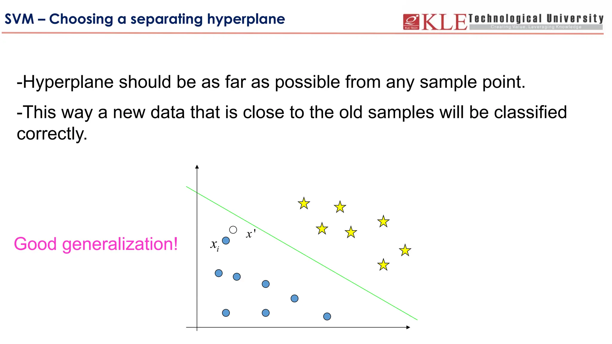
-Hyperplane should be as far as possible from any sample point.
-This way a new data that is close to the old samples will be classified
correctly.
Good generalization!

51. SVM – Choosing a separating hyperplane
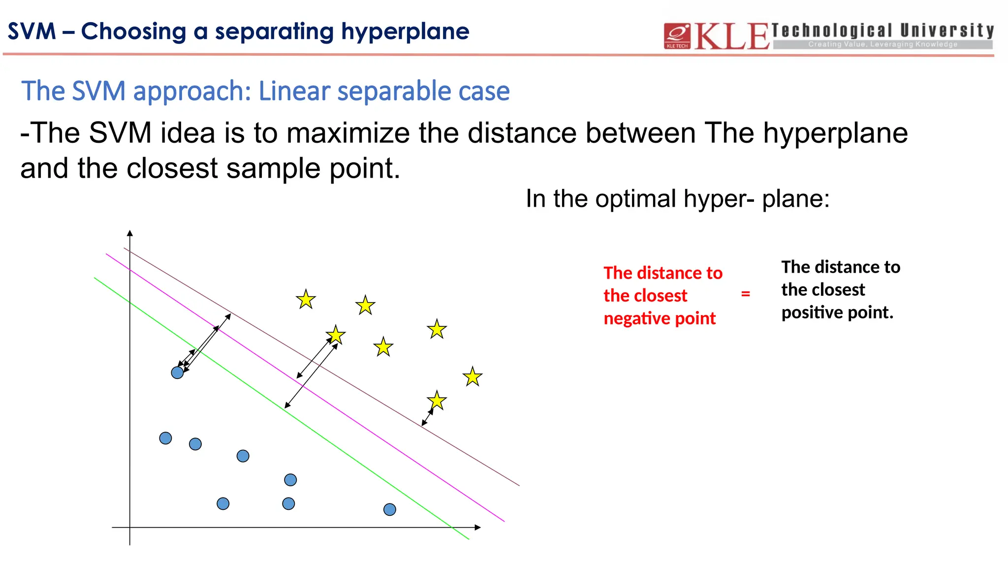
The SVM approach: Linear separable case
-The SVM idea is to maximize the distance between The hyperplane
and the closest sample point.
In the optimal hyper- plane:
The distance to
the closest
negative point
The distance to
the closest
positive point.
=

52. SVM – Choosing a separating hyperplane
i
x
M
a
r
g
i
n
d
d
d
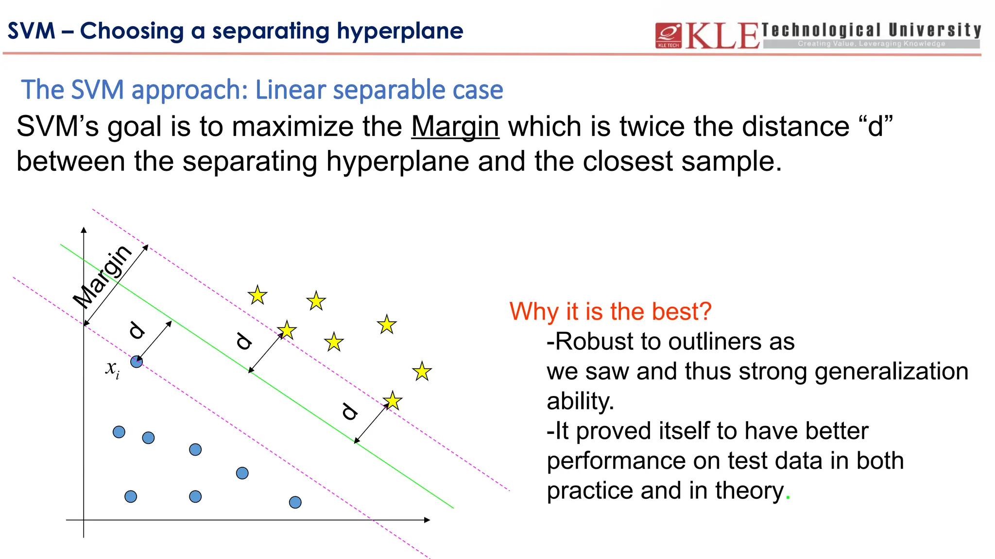
SVM’s goal is to maximize the Margin which is twice the distance “d”
between the separating hyperplane and the closest sample.
Why it is the best?
-Robust to outliners as
we saw and thus strong generalization
ability.
-It proved itself to have better
performance on test data in both
practice and in theory.
The SVM approach: Linear separable case

53. SVM – Choosing a separating hyperplane
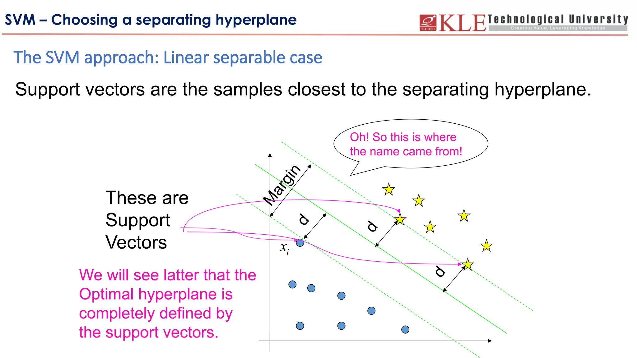
The SVM approach: Linear separable case
i
x
M
a
r
g
i
n
d
d
d
These are
Support
Vectors
Support vectors are the samples closest to the separating hyperplane.
We will see latter that the
Optimal hyperplane is
completely defined by
the support vectors.
Oh! So this is where
the name came from!

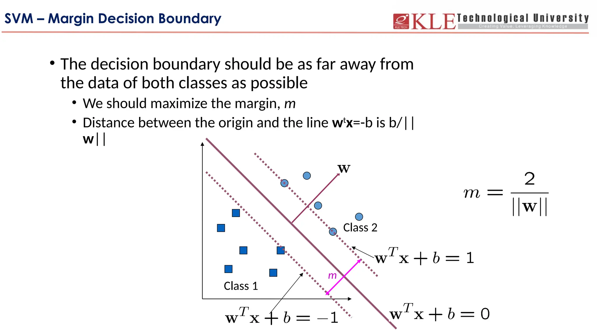
54. SVM – Margin Decision Boundary
• The decision boundary should be as far away from
the data of both classes as possible
• We should maximize the margin, m
• Distance between the origin and the line wt
x=-b is b/||
w||
Class 1
Class 2
m

55. SVM - Example

56. SVM - Example

57. SVM - Example

58. SVM - Example

59. SVM - Example

60. SVM - Example

61. SVM - Example

62. SVM - Example

63. SVM - Example

64. Decision Tree and Naïve
Bayesian

65. Decision Tree

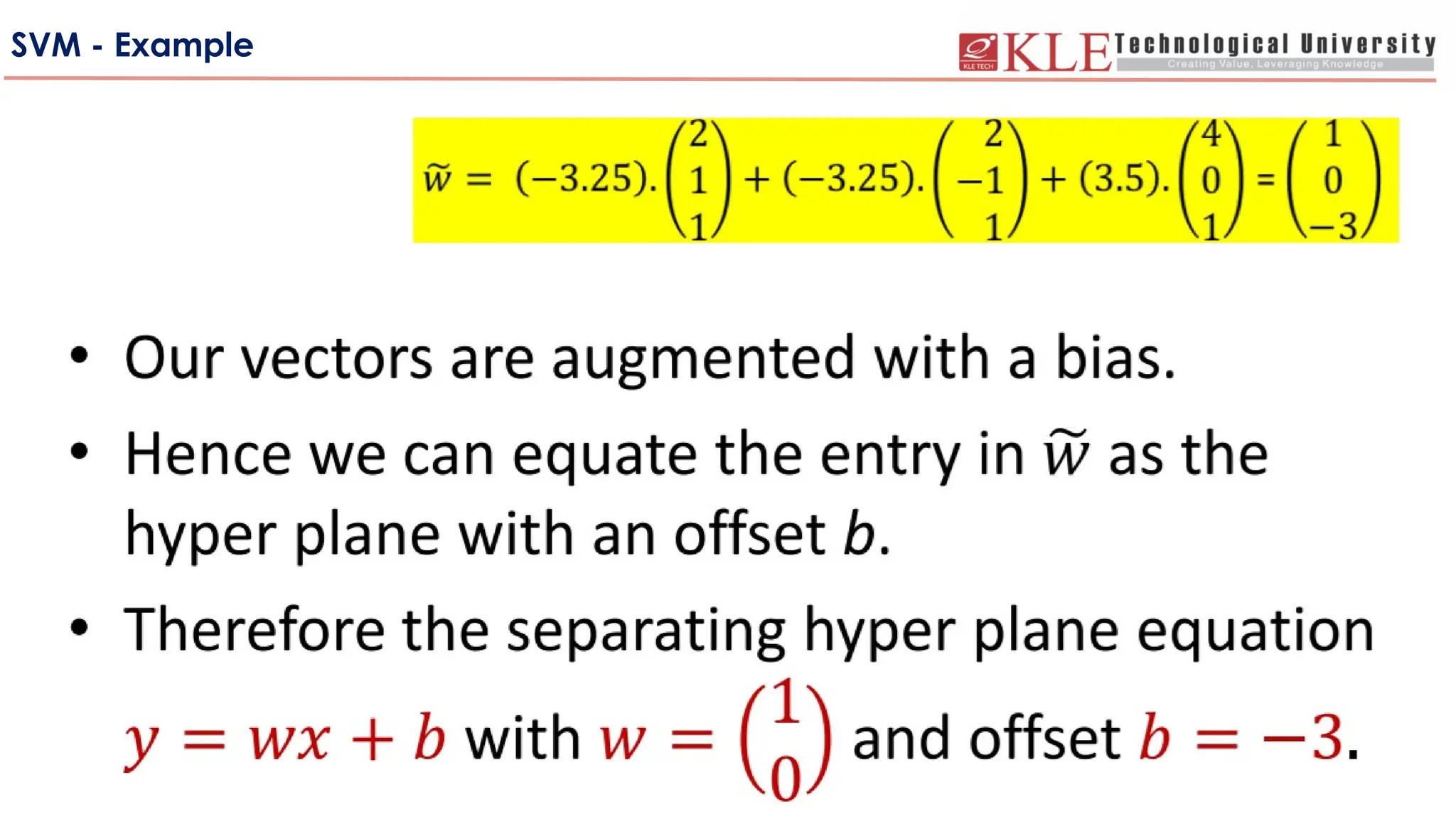
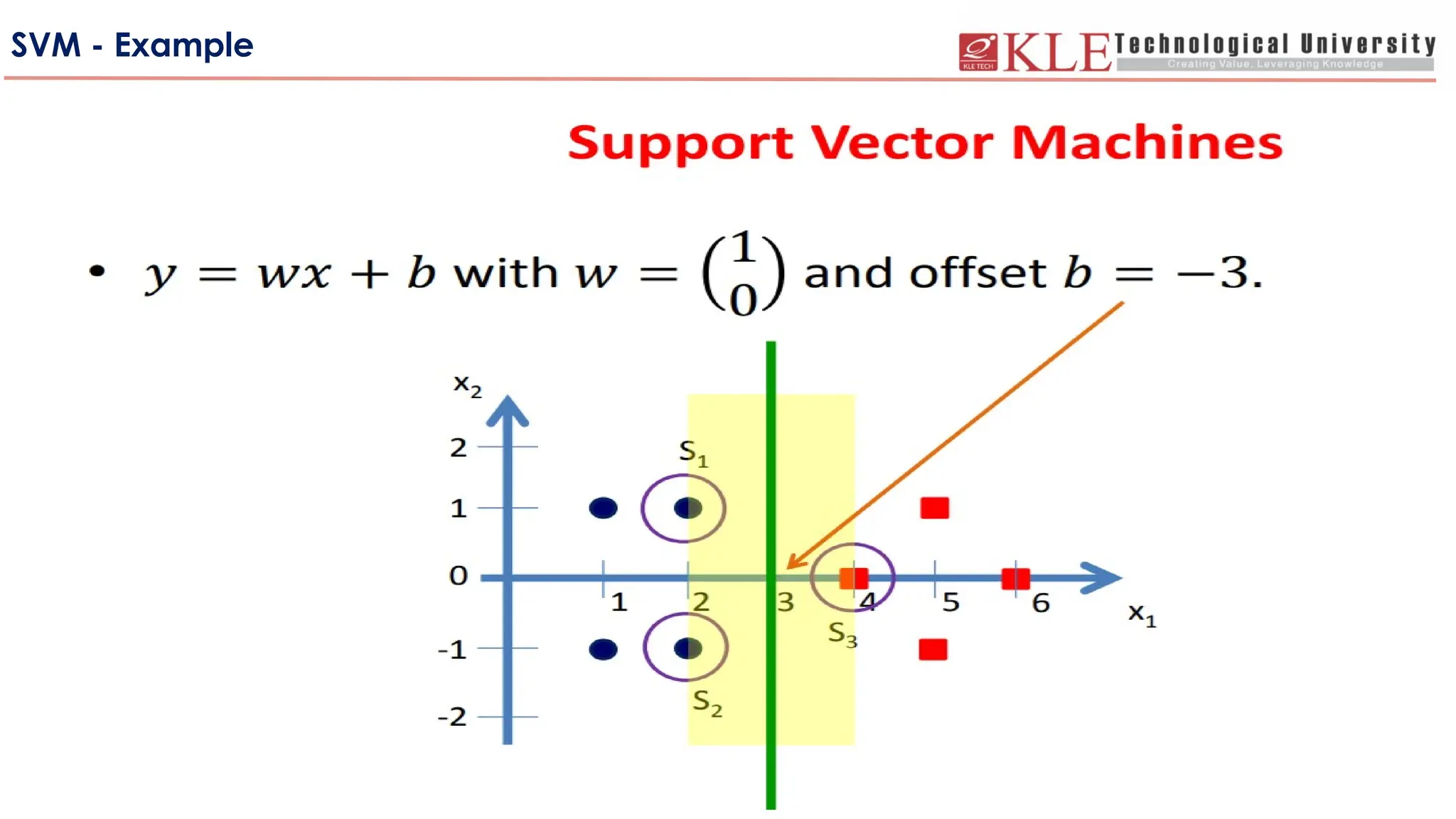
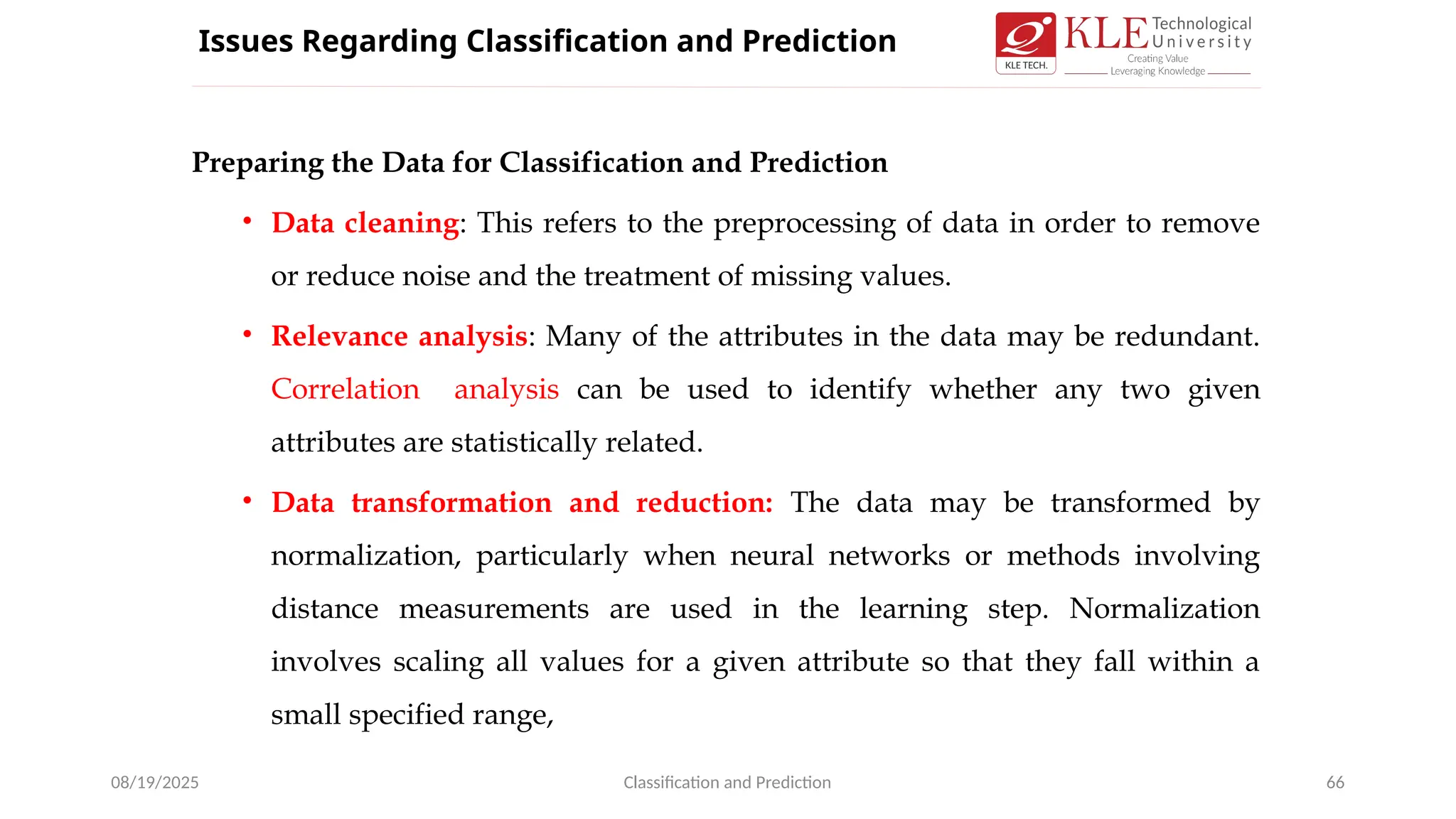
66. Preparing the Data for Classification and Prediction
• Data cleaning: This refers to the preprocessing of data in order to remove
or reduce noise and the treatment of missing values.
• Relevance analysis: Many of the attributes in the data may be redundant.
Correlation analysis can be used to identify whether any two given
attributes are statistically related.
• Data transformation and reduction: The data may be transformed by
normalization, particularly when neural networks or methods involving
distance measurements are used in the learning step. Normalization
involves scaling all values for a given attribute so that they fall within a
small specified range,
08/19/2025 Classification and Prediction 66
Issues Regarding Classification and Prediction

67. • Accuracy: The accuracy of a classifier refers to the ability of a given
classifier to correctly predict the class label of new or previously unseen
data (i.e., tuples without class label information).
• Speed: This refers to the computational costs involved in generating and
using the given classifier or predictor
• Robustness: This is the ability of the classifier or predictor to make
correct predictions given noisy data or data with missing values.
• Scalability: This refers to the ability to construct the classifier or
predictor efficiently given large amounts of data.
08/19/2025 Classification and Prediction 67
Comparing Classification and Prediction
Methods

68. • Decision tree
• A flow-chart-like tree structure
• Internal node denotes a test on an attribute
• Branch represents an outcome of the test
• Leaf nodes represent class labels or class distribution
• Decision tree generation consists of two phases
• Tree construction
• At start, all the training examples are at the root
• Partition examples recursively based on selected attributes
• Tree pruning
• Identify and remove branches that reflect noise or outliers
• Use of decision tree: Classifying an unknown sample
• Test the attribute values of the sample against the decision tree
Classification by decision tree Induction

69. 08/19/2025 Classification and Prediction 69
Training Dataset

70. • Basic algorithm (a greedy algorithm)
• Tree is constructed in a top-down recursive divide-and-conquer manner
• At start, all the training examples are at the root
• Attributes are categorical (if continuous-valued, they are discretized in
advance)
• Examples are partitioned recursively based on selected attributes
• Test attributes are selected on the basis of a heuristic or statistical
measure (e.g., information gain)
• Conditions for stopping partitioning
• All samples for a given node belong to the same class
• There are no remaining attributes for further partitioning – majority
voting is employed for classifying the leaf
• There are no samples left
Algorithm

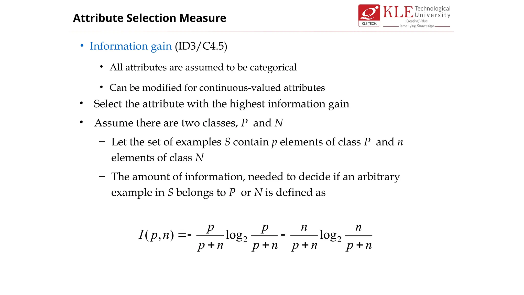
71. • Information gain (ID3/C4.5)
• All attributes are assumed to be categorical
• Can be modified for continuous-valued attributes
Attribute Selection Measure
• Select the attribute with the highest information gain
• Assume there are two classes, P and N
– Let the set of examples S contain p elements of class P and n
elements of class N
– The amount of information, needed to decide if an arbitrary
example in S belongs to P or N is defined as
n
p
n
n
p
n
n
p
p
n
p
p
n
p
I






 2
2 log
log
)
,
(

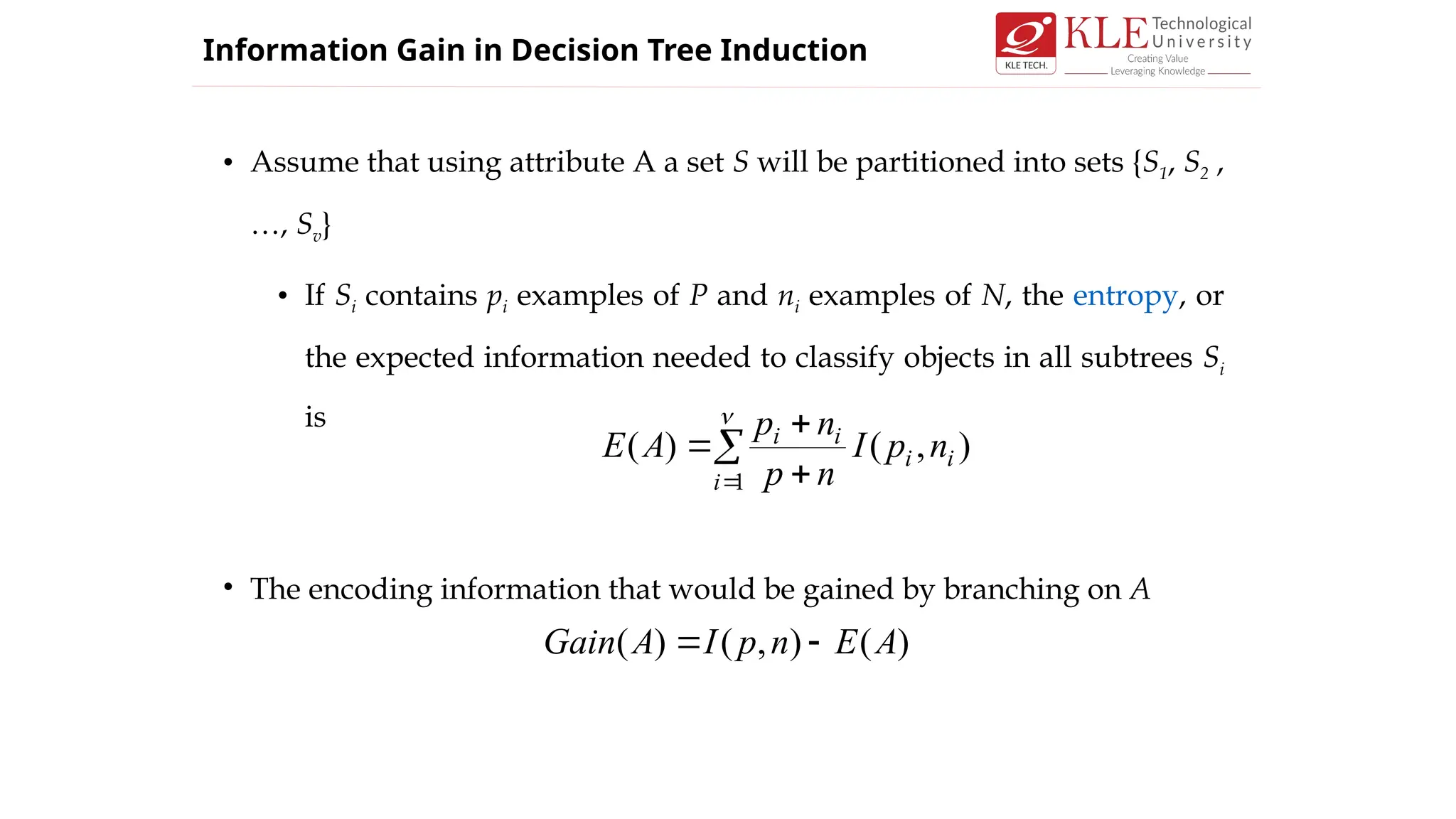
72. • Assume that using attribute A a set S will be partitioned into sets {S1, S2 ,
…, Sv}
• If Si contains pi examples of P and ni examples of N, the entropy, or
the expected information needed to classify objects in all subtrees Si
is
• The encoding information that would be gained by branching on A

 



1
)
,
(
)
(
i
i
i
i
i
n
p
I
n
p
n
p
A
E
)
(
)
,
(
)
( A
E
n
p
I
A
Gain 

Information Gain in Decision Tree Induction

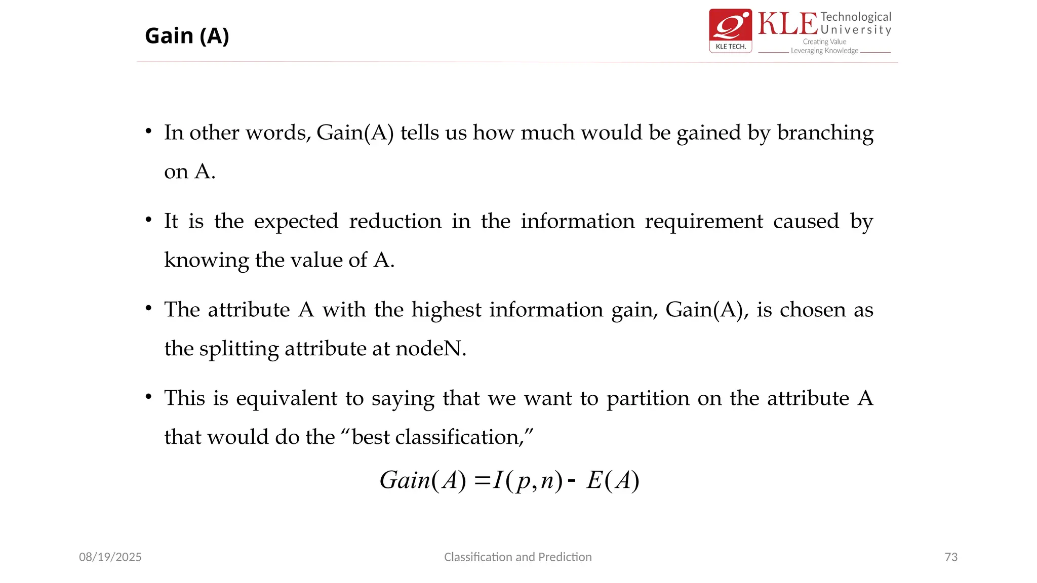
73. • In other words, Gain(A) tells us how much would be gained by branching
on A.
• It is the expected reduction in the information requirement caused by
knowing the value of A.
• The attribute A with the highest information gain, Gain(A), is chosen as
the splitting attribute at nodeN.
• This is equivalent to saying that we want to partition on the attribute A
that would do the “best classification,”
08/19/2025 Classification and Prediction 73
Gain (A)
)
(
)
,
(
)
( A
E
n
p
I
A
Gain 


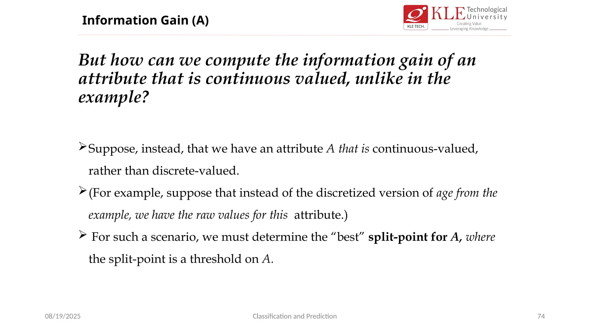
74. But how can we compute the information gain of an
attribute that is continuous valued, unlike in the
example?
08/19/2025 Classification and Prediction 74
Suppose, instead, that we have an attribute A that is continuous-valued,
rather than discrete-valued.
(For example, suppose that instead of the discretized version of age from the
example, we have the raw values for this attribute.)
 For such a scenario, we must determine the “best” split-point for A, where
the split-point is a threshold on A.
Information Gain (A)

75. • The algorithm is called with three parameters: D, attribute list, and Attribute
selection method.
• We refer to D as a data partition. Initially, it is the complete set of training tuples
and their associated class labels.
• The parameter attribute list is a list of attributes describing the tuples.
• Attribute selection method specifies a heuristic procedure for selecting the
attribute that “best” discriminates the given tuples according to class.
08/19/2025 Classification and Prediction 75
Information Gain in Decision Tree Induction

76. • Is a heuristic for selecting the splitting criterion that “best” separates a given
data partition, D, of class-labeled training tuples into individual classes.
• If we were to split D into smaller partitions according to the outcomes of the
splitting criterion, ideally each partition would be pure.
• Attribute selection measures are also known as splitting rules because they
determine how the tuples at a given node are to be split.
08/19/2025 Classification and Prediction 76
Attribute Selection Measures

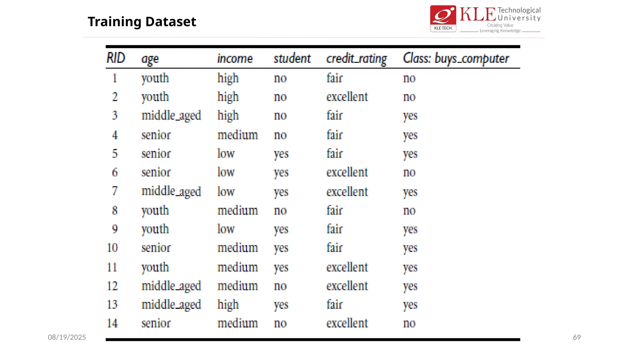
77. The class label attribute, buys computer, has two distinct values (namely,
yes, no)
Therefore, there are two distinct classes (that is, m = 2).
Let class C1 correspond to yes.
Let class C2 correspond to no.
There are
Nine tuples of class yes
Five tuples of class no.
A (root) node N is created for the tuples in D.
To find the splitting criterion for these tuples, we must compute the
information gain of each attribute.
Implementation

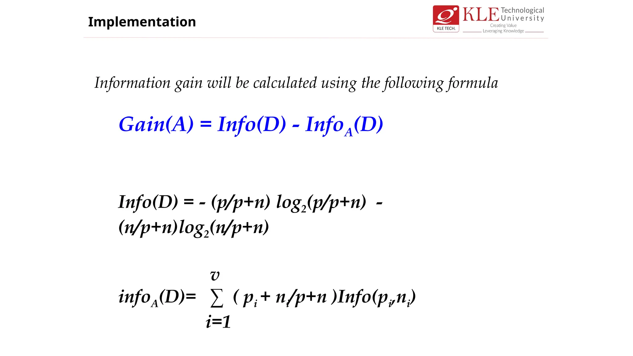
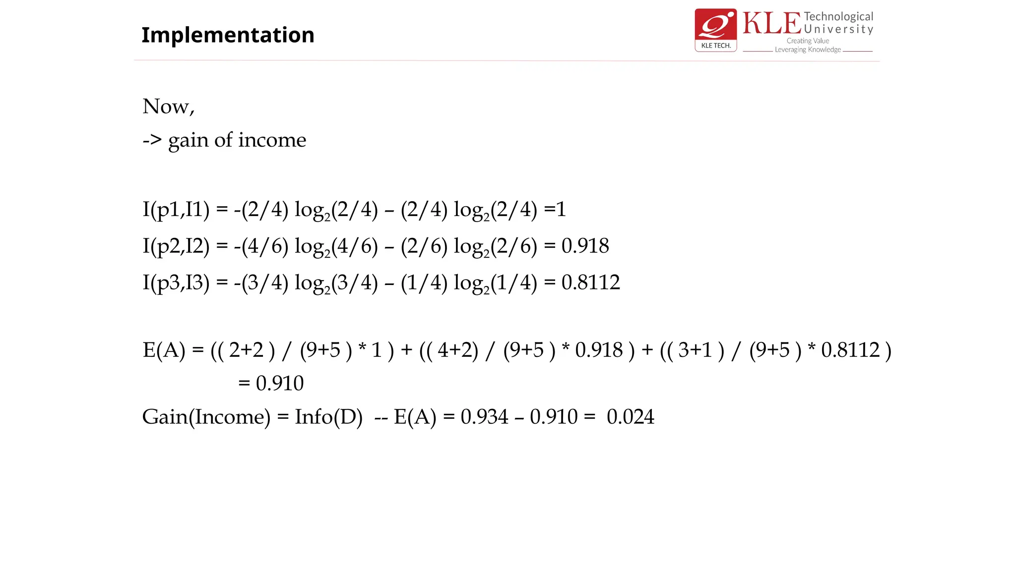
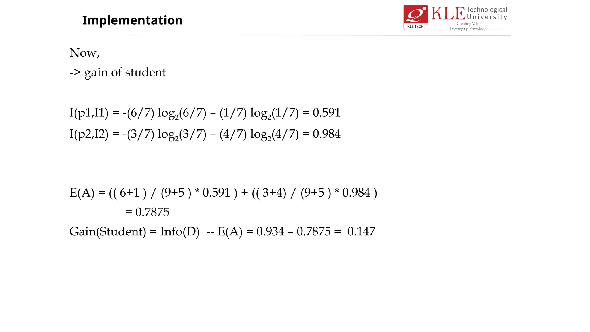
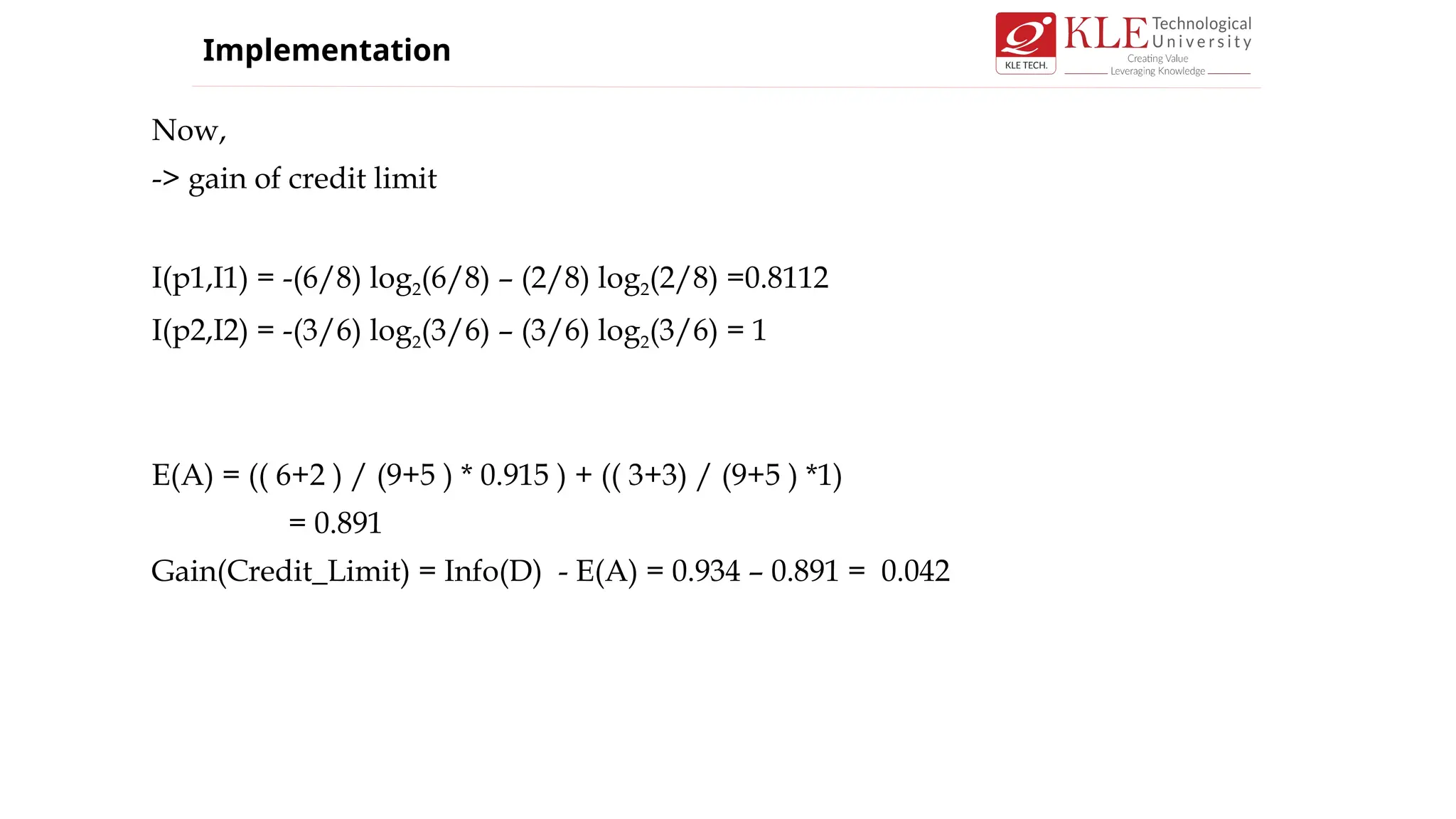
78. Information gain will be calculated using the following formula
Gain(A) = Info(D) - InfoA(D)
Info(D) = - (p/p+n) log2(p/p+n) -
(n/p+n)log2(n/p+n)
v
infoA(D)= ∑ ( pi + ni/p+n )Info(pi,ni)
i=1
Implementation

79. Info(D) = -9/14 log2(9/14) –(5/14)log2(5/14)
= 0.409 + 0.530
= 0.934
Now,
-> gain for age,
I(p1,I1) = -(2/5) log2(2/5) – (3/5) log2(3/5) = 0.971
I(p2,I2) = -(4/4) log2(4/4) – (0/4) log2(0/4) = 0
I(p3,I3) = -(3/5) log2(3/5) – (2/5) log2(2/5) = 0.971
E(A) = (( 2+3 ) / (9+5 ) * 0.971 ) + (( 4+0 ) / (9+5 ) * 0 ) + (( 3+2 ) / (9+5 ) * 0.971 )
= 0.694
Gain(Age) = Info(D) -- E(A) = 0.934 – 0.694 = 0.240
Implementation

80. Now,
-> gain of income
I(p1,I1) = -(2/4) log2(2/4) – (2/4) log2(2/4) =1
I(p2,I2) = -(4/6) log2(4/6) – (2/6) log2(2/6) = 0.918
I(p3,I3) = -(3/4) log2(3/4) – (1/4) log2(1/4) = 0.8112
E(A) = (( 2+2 ) / (9+5 ) * 1 ) + (( 4+2) / (9+5 ) * 0.918 ) + (( 3+1 ) / (9+5 ) * 0.8112 )
= 0.910
Gain(Income) = Info(D) -- E(A) = 0.934 – 0.910 = 0.024
Implementation

81. Now,
-> gain of student
I(p1,I1) = -(6/7) log2(6/7) – (1/7) log2(1/7) = 0.591
I(p2,I2) = -(3/7) log2(3/7) – (4/7) log2(4/7) = 0.984
E(A) = (( 6+1 ) / (9+5 ) * 0.591 ) + (( 3+4) / (9+5 ) * 0.984 )
= 0.7875
Gain(Student) = Info(D) -- E(A) = 0.934 – 0.7875 = 0.147
Implementation

82. Now,
-> gain of credit limit
I(p1,I1) = -(6/8) log2(6/8) – (2/8) log2(2/8) =0.8112
I(p2,I2) = -(3/6) log2(3/6) – (3/6) log2(3/6) = 1
E(A) = (( 6+2 ) / (9+5 ) * 0.915 ) + (( 3+3) / (9+5 ) *1)
= 0.891
Gain(Credit_Limit) = Info(D) - E(A) = 0.934 – 0.891 = 0.042
Implementation

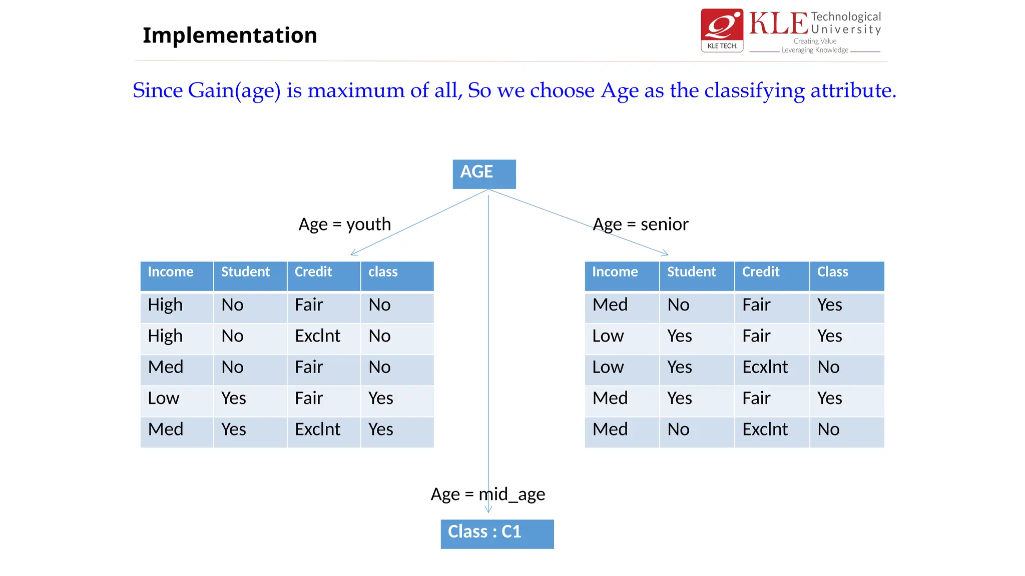
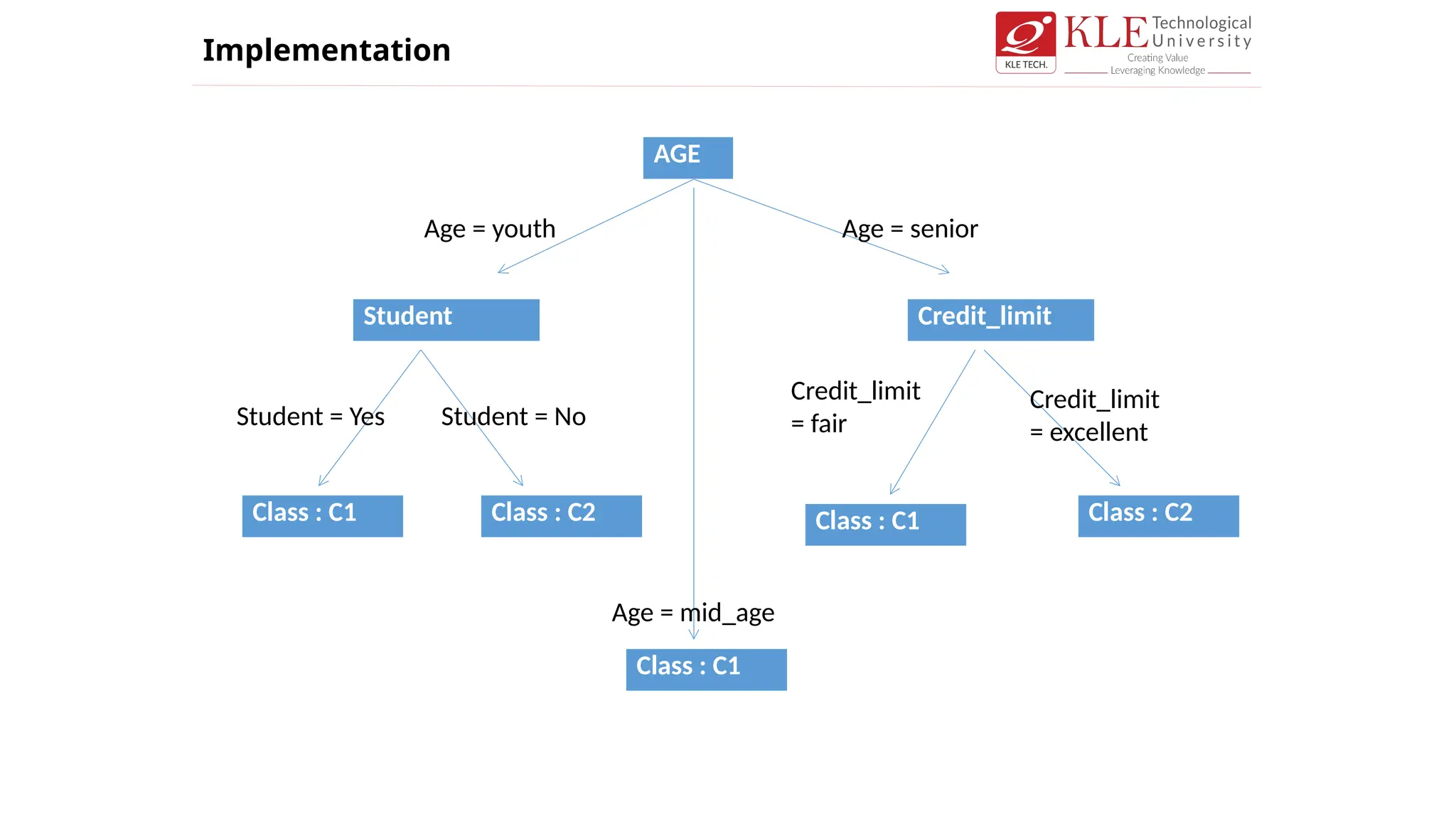
83. Since Gain(age) is maximum of all, So we choose Age as the classifying attribute.
Implementation
Income Student Credit class
High No Fair No
High No Exclnt No
Med No Fair No
Low Yes Fair Yes
Med Yes Exclnt Yes
Income Student Credit Class
Med No Fair Yes
Low Yes Fair Yes
Low Yes Ecxlnt No
Med Yes Fair Yes
Med No Exclnt No
AGE
Class : C1
Age = youth Age = senior
Age = mid_age

84. AGE
Class : C1
Age = youth Age = senior
Age = mid_age
Student Credit_limit
Class : C2
Class : C1 Class : C1 Class : C2
Student = Yes Student = No
Credit_limit
= fair
Credit_limit
= excellent
Implementation

85. 08/19/2025 Classification and Prediction 85
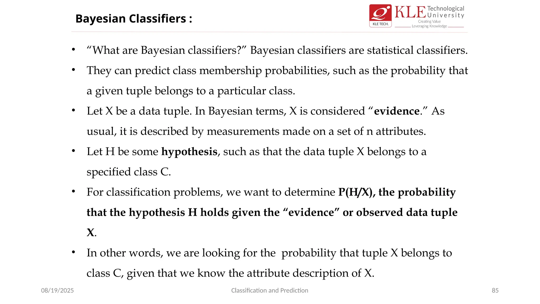
• “What are Bayesian classifiers?” Bayesian classifiers are statistical classifiers.
• They can predict class membership probabilities, such as the probability that
a given tuple belongs to a particular class.
• Let X be a data tuple. In Bayesian terms, X is considered “evidence.” As
usual, it is described by measurements made on a set of n attributes.
• Let H be some hypothesis, such as that the data tuple X belongs to a
specified class C.
• For classification problems, we want to determine P(H/X), the probability
that the hypothesis H holds given the “evidence” or observed data tuple
X.
• In other words, we are looking for the probability that tuple X belongs to
class C, given that we know the attribute description of X.
Bayesian Classifiers :

86. 08/19/2025 Classification and Prediction 86
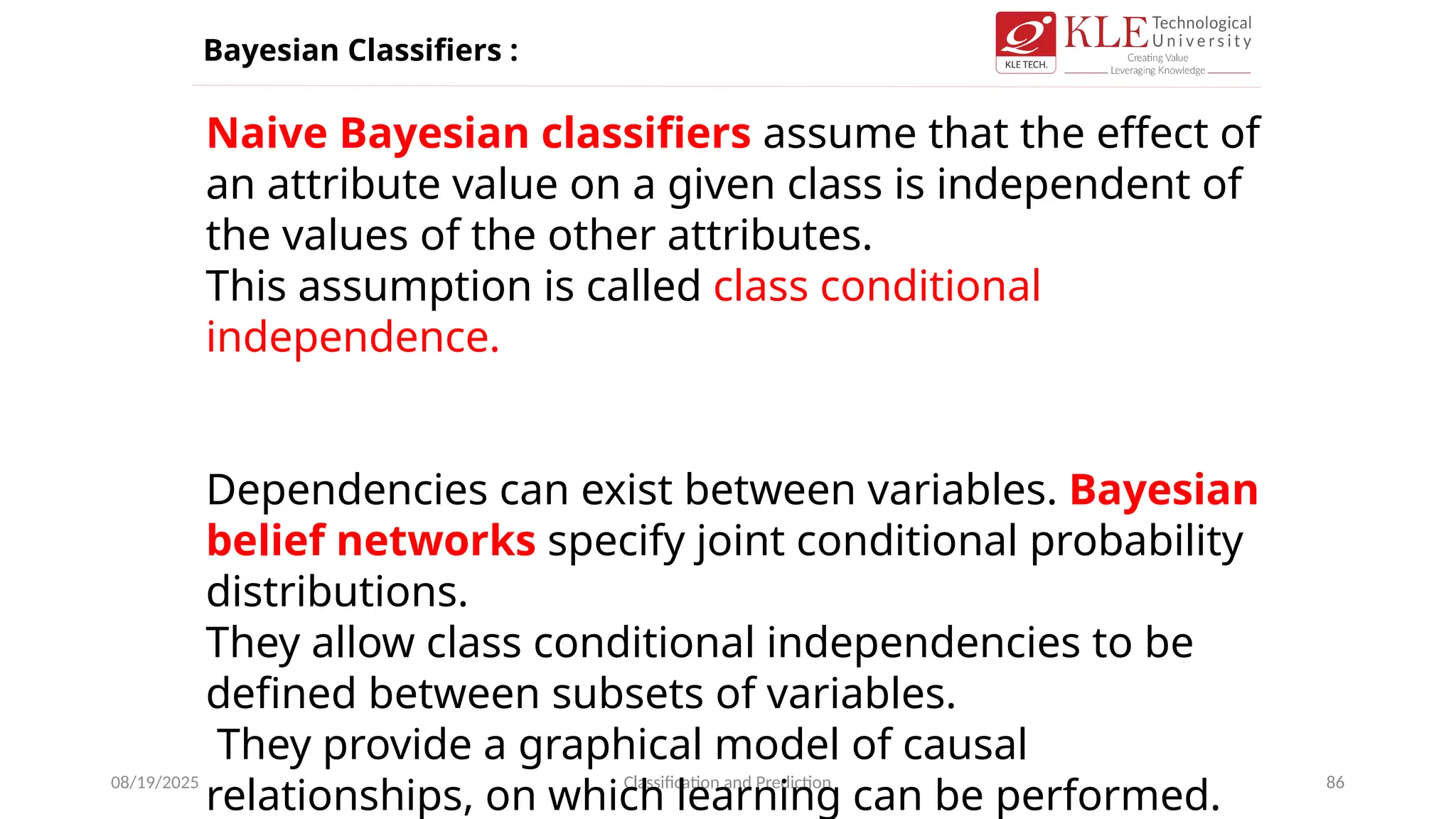
Naive Bayesian classifiers assume that the effect of
an attribute value on a given class is independent of
the values of the other attributes.
This assumption is called class conditional
independence.
Dependencies can exist between variables. Bayesian
belief networks specify joint conditional probability
distributions.
They allow class conditional independencies to be
defined between subsets of variables.
They provide a graphical model of causal
relationships, on which learning can be performed.
Bayesian Classifiers :

87. August 19, 2025 Data Mining: Concepts and Techniques 87
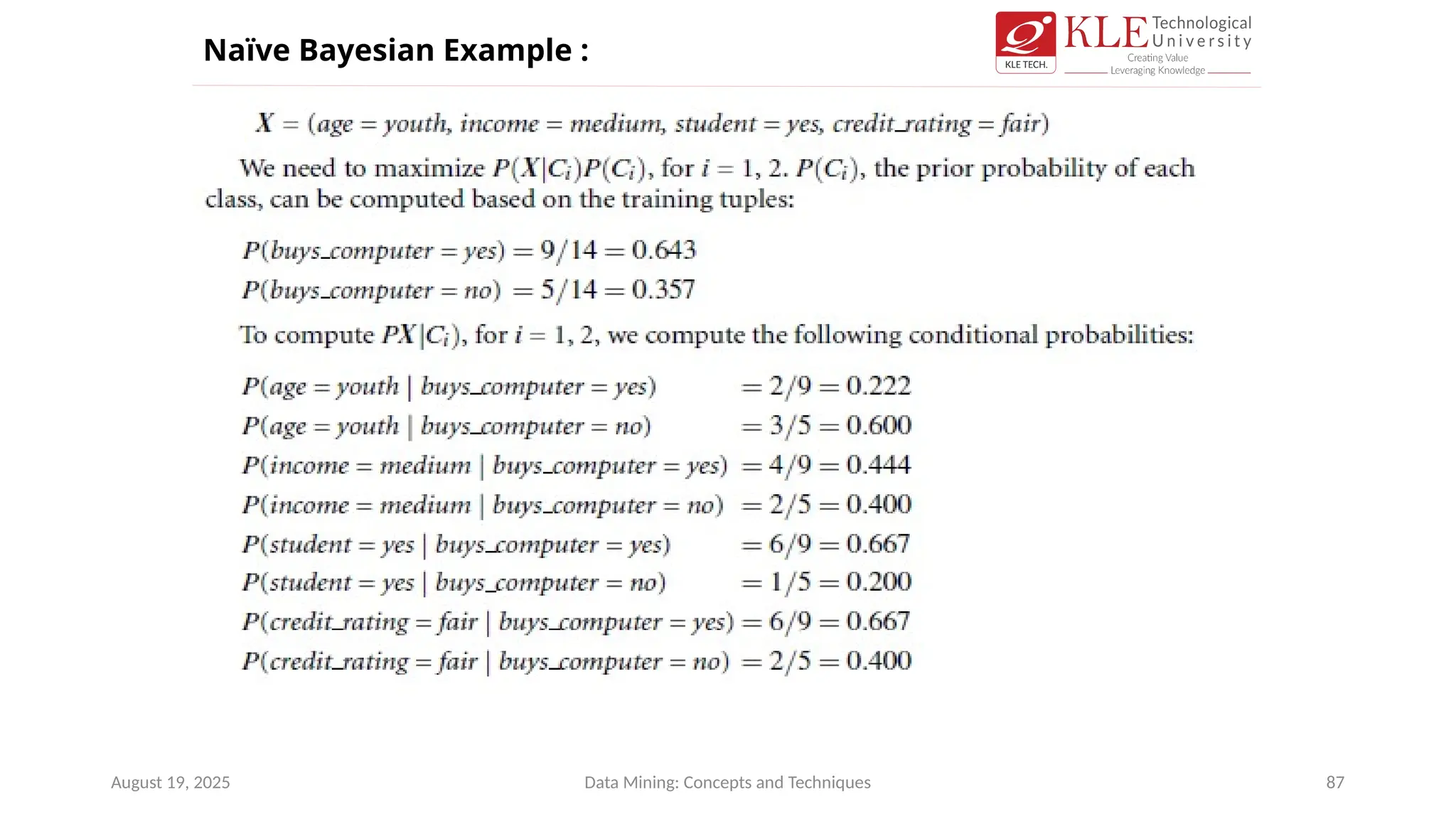
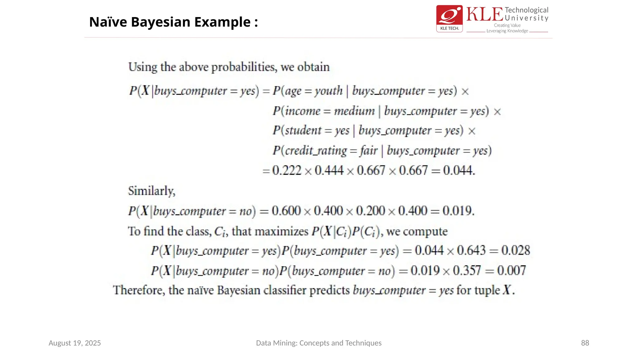
Naïve Bayesian Example :

88. August 19, 2025 Data Mining: Concepts and Techniques 88
Naïve Bayesian Example :