The document discusses numerical differentiation, which is used to approximate derivatives of functions when only tabulated data is available. It presents the forward, backward, and central difference formulas for approximating the first derivative. The central difference formula provides more accurate approximations, with errors on the order of h^2 rather than h. The document also shows an example applying the formulas to estimate the derivative of a sample function at different points using various step sizes h. Halving h reduces the error as expected based on the formulas.

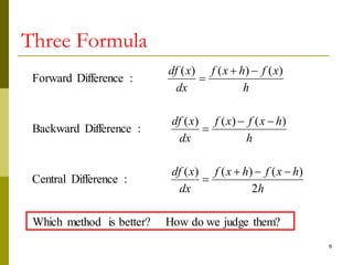
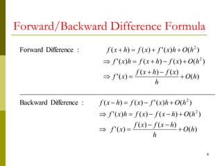
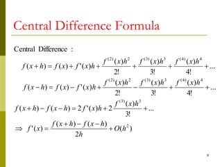
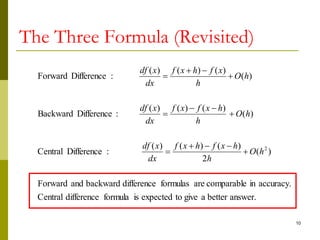
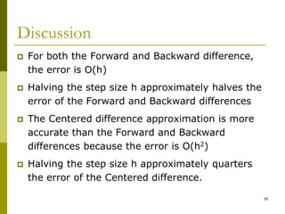
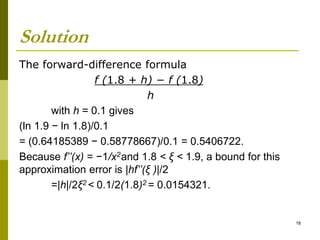
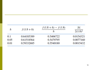
1. 1
Numerical Differentiation

2. 2
Numerical Differentiation
 First order derivatives
 High order derivatives
Examples

3. 3
Motivation
 How do you evaluate the
derivative of a tabulated
function.
 How do we determine the
velocity and acceleration
from tabulated
measurements.
Time
(second)
Displacement
(meters)
0 30.1
5 48.2
10 50.0
15 40.2

4. 4
Recall
n
n
n
n
h
h
E
h
h
C
E
that
such
C
finite
real
h
O
E
h
O
h
x
f
h
x
f
h
x
f
x
f
h
x
f
h
x
f
h
x
f
dx
df
similar to
rate
at
zero
g
approachin
is
order
of
is
E
:
,
,
)
(
)
(
!
3
)
(
!
2
)
(
)
(
'
)
(
)
(
:
Theorem
Taylor
)
(
)
(
lim
4
3
)
3
(
2
)
2
(
0
















5. For small values of h, the difference quotient [f (x0 + h) − f (x0)]/h
can be used to approximate f’(x0) with an error bounded by M|h|/2,
where M is a bound on |f’’(x)| for x between x0 and x0 +h.
CISE301_Topic6 5

6. 6
Three Formula
them?
judge
we
do
How
better?
is
method
Which
2
)
(
)
(
)
(
:
Difference
Central
)
(
)
(
)
(
:
Difference
Backward
)
(
)
(
)
(
:
Difference
Forward
h
h
x
f
h
x
f
dx
x
df
h
h
x
f
x
f
dx
x
df
h
x
f
h
x
f
dx
x
df











7. 7
The Three Formulas

8. 8
Forward/Backward Difference Formula
)
(
)
(
)
(
)
(
'
)
(
)
(
)
(
)
(
'
)
(
)
(
'
)
(
)
(
:
Difference
Backward
_____
__________
__________
__________
__________
__________
)
(
)
(
)
(
)
(
'
)
(
)
(
)
(
)
(
'
)
(
)
(
'
)
(
)
(
:
Difference
Forward
2
2
2
2
h
O
h
h
x
f
x
f
x
f
h
O
h
x
f
x
f
h
x
f
h
O
h
x
f
x
f
h
x
f
h
O
h
x
f
h
x
f
x
f
h
O
x
f
h
x
f
h
x
f
h
O
h
x
f
x
f
h
x
f





























9. 9
Central Difference Formula
)
(
2
)
(
)
(
)
(
'
...
!
3
)
(
2
)
(
'
2
)
(
)
(
...
!
4
)
(
!
3
)
(
!
2
)
(
)
(
'
)
(
)
(
...
!
4
)
(
!
3
)
(
!
2
)
(
)
(
'
)
(
)
(
:
Difference
Central
2
3
)
3
(
4
)
4
(
3
)
3
(
2
)
2
(
4
)
4
(
3
)
3
(
2
)
2
(
h
O
h
h
x
f
h
x
f
x
f
h
x
f
h
x
f
h
x
f
h
x
f
h
x
f
h
x
f
h
x
f
h
x
f
x
f
h
x
f
h
x
f
h
x
f
h
x
f
h
x
f
x
f
h
x
f



























10. 10
The Three Formula (Revisited)
answer.
better
a
give
to
expected
is
formula
difference
Central
accuracy.
in
comparable
are
formulas
difference
backward
and
Forward
)
(
2
)
(
)
(
)
(
:
Difference
Central
)
(
)
(
)
(
)
(
:
Difference
Backward
)
(
)
(
)
(
)
(
:
Difference
Forward
2
h
O
h
h
x
f
h
x
f
dx
x
df
h
O
h
h
x
f
x
f
dx
x
df
h
O
h
x
f
h
x
f
dx
x
df














11. 11
Higher Order Formulas
12
)
(
)
(
)
(
)
(
2
)
(
)
(
...
!
4
)
(
2
!
2
)
(
2
)
(
2
)
(
)
(
...
!
4
)
(
!
3
)
(
!
2
)
(
)
(
'
)
(
)
(
...
!
4
)
(
!
3
)
(
!
2
)
(
)
(
'
)
(
)
(
2
)
4
(
2
2
)
2
(
4
)
4
(
2
)
2
(
4
)
4
(
3
)
3
(
2
)
2
(
4
)
4
(
3
)
3
(
2
)
2
(
h
f
Error
h
O
h
h
x
f
x
f
h
x
f
x
f
h
x
f
h
x
f
x
f
h
x
f
h
x
f
h
x
f
h
x
f
h
x
f
h
x
f
x
f
h
x
f
h
x
f
h
x
f
h
x
f
h
x
f
x
f
h
x
f
































12. 12
Other Higher Order Formulas
.
order
error
the
obtain
and
them
prove
to
Theorem
Taylor
use
can
You
possible.
also
are
)...
(
),
(
for
formulas
Other
)
(
with
Formulas
Central
)
2
(
)
(
4
)
(
6
)
(
4
)
2
(
)
(
2
)
2
(
)
(
2
)
(
2
)
2
(
)
(
)
(
)
(
2
)
(
)
(
)
3
(
)
2
(
2
4
)
4
(
3
)
3
(
2
)
2
(
x
f
x
f
h
O
Error
h
h
x
f
h
x
f
x
f
h
x
f
h
x
f
x
f
h
h
x
f
h
x
f
h
x
f
h
x
f
x
f
h
h
x
f
x
f
h
x
f
x
f
























13. Example
 Use forward, backward and centered difference
approximations to estimate the first derivate of:
f(x) = –0.1x4 – 0.15x3 – 0.5x2 – 0.25x + 1.2
at x = 0.5 using step size h = 0.5 and h = 0.25
 Note that the derivate can be obtained directly:
f’(x) = –0.4x3 – 0.45x2 – 1.0x – 0.25
The true value of f’(0.5) = -0.9125
 In this example, the function and its derivate
are known. However, in general, only tabulated
data might be given.
13

14. Solution with Step Size = 0.5
 f(0.5) = 0.925, f(0) = 1.2, f(1.0) = 0.2
 Forward Divided Difference:
f’(0.5)  (0.2 – 0.925)/0.5 = -1.45
|t| = |(-0.9125+1.45)/-0.9125| = 58.9%
 Backward Divided Difference:
f’(0.5)  (0.925 – 1.2)/0.5 = -0.55
|t| = |(-0.9125+0.55)/-0.9125| = 39.7%
 Centered Divided Difference:
f’(0.5)  (0.2 – 1.2)/1.0 = -1.0
|t| = |(-0.9125+1.0)/-0.9125| = 9.6%
14

15. Solution with Step Size = 0.25
 f(0.5)=0.925, f(0.25)=1.1035, f(0.75)=0.6363
 Forward Divided Difference:
f’(0.5)  (0.6363 – 0.925)/0.25 = -1.155
|t| = |(-0.9125+1.155)/-0.9125| = 26.5%
 Backward Divided Difference:
f’(0.5)  (0.925 – 1.1035)/0.25 = -0.714
|t| = |(-0.9125+0.714)/-0.9125| = 21.7%
 Centered Divided Difference:
f’(0.5)  (0.6363 – 1.1035)/0.5 = -0.934
|t| = |(-0.9125+0.934)/-0.9125| = 2.4%
15

16. Discussion
 For both the Forward and Backward difference,
the error is O(h)
 Halving the step size h approximately halves the
error of the Forward and Backward differences
 The Centered difference approximation is more
accurate than the Forward and Backward
differences because the error is O(h2)
 Halving the step size h approximately quarters
the error of the Centered difference.
16

17. Use the forward-difference formula to approximate the
derivative of f (x) = ln x at x0 = 1.8 using h = 0.1, h =
0.05, and h = 0.01, and determine bounds for the
approximation errors.
17
Example 2

18. Solution
The forward-difference formula
f (1.8 + h) − f (1.8)
h
with h = 0.1 gives
(ln 1.9 − ln 1.8)/0.1
= (0.64185389 − 0.58778667)/0.1 = 0.5406722.
Because f’’(x) = −1/x2and 1.8 < ξ < 1.9, a bound for this
approximation error is |hf’’(ξ )|/2
=|h|/2ξ2 < 0.1/2(1.8)2 = 0.0154321.
18

19. 19