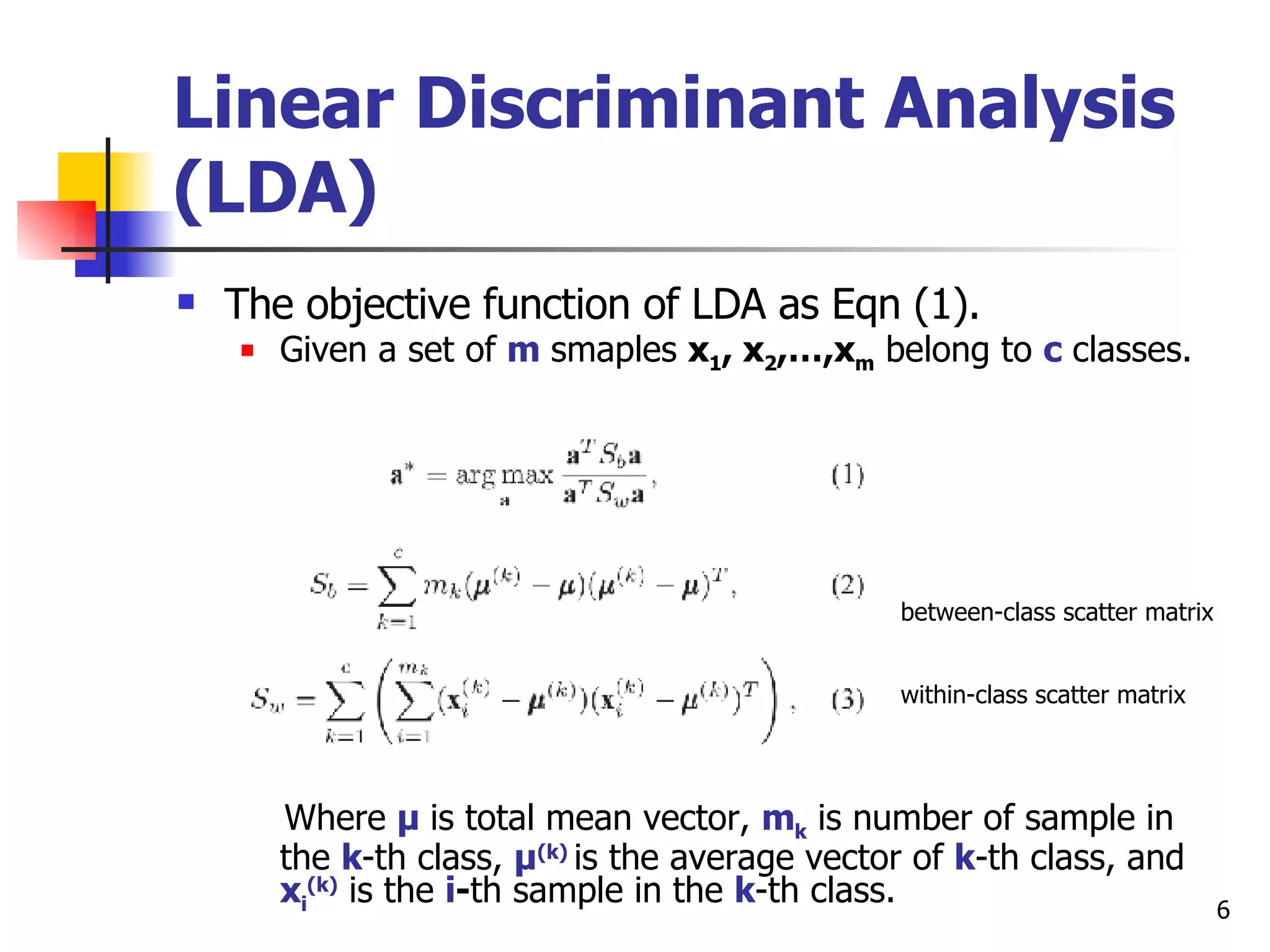
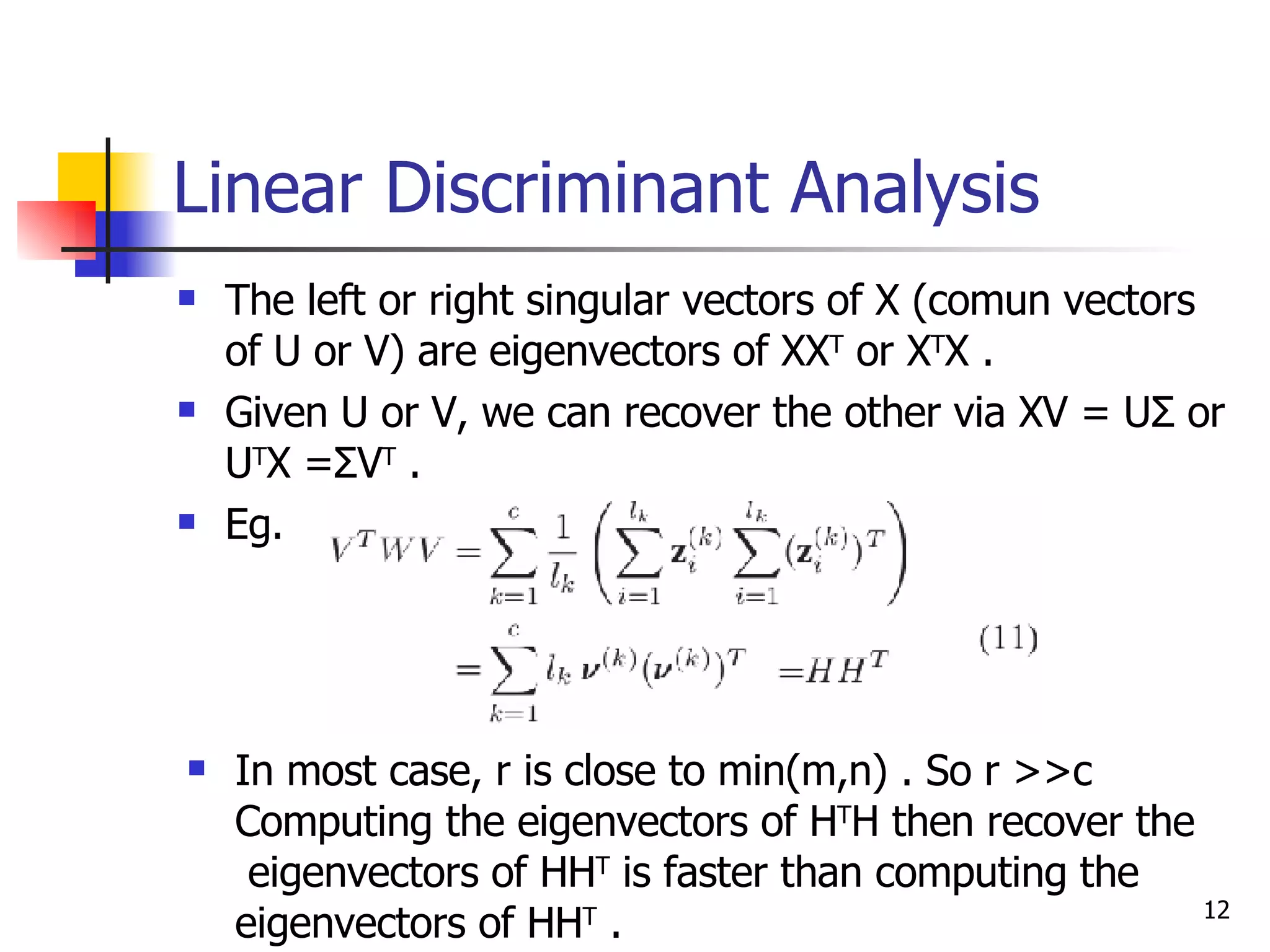
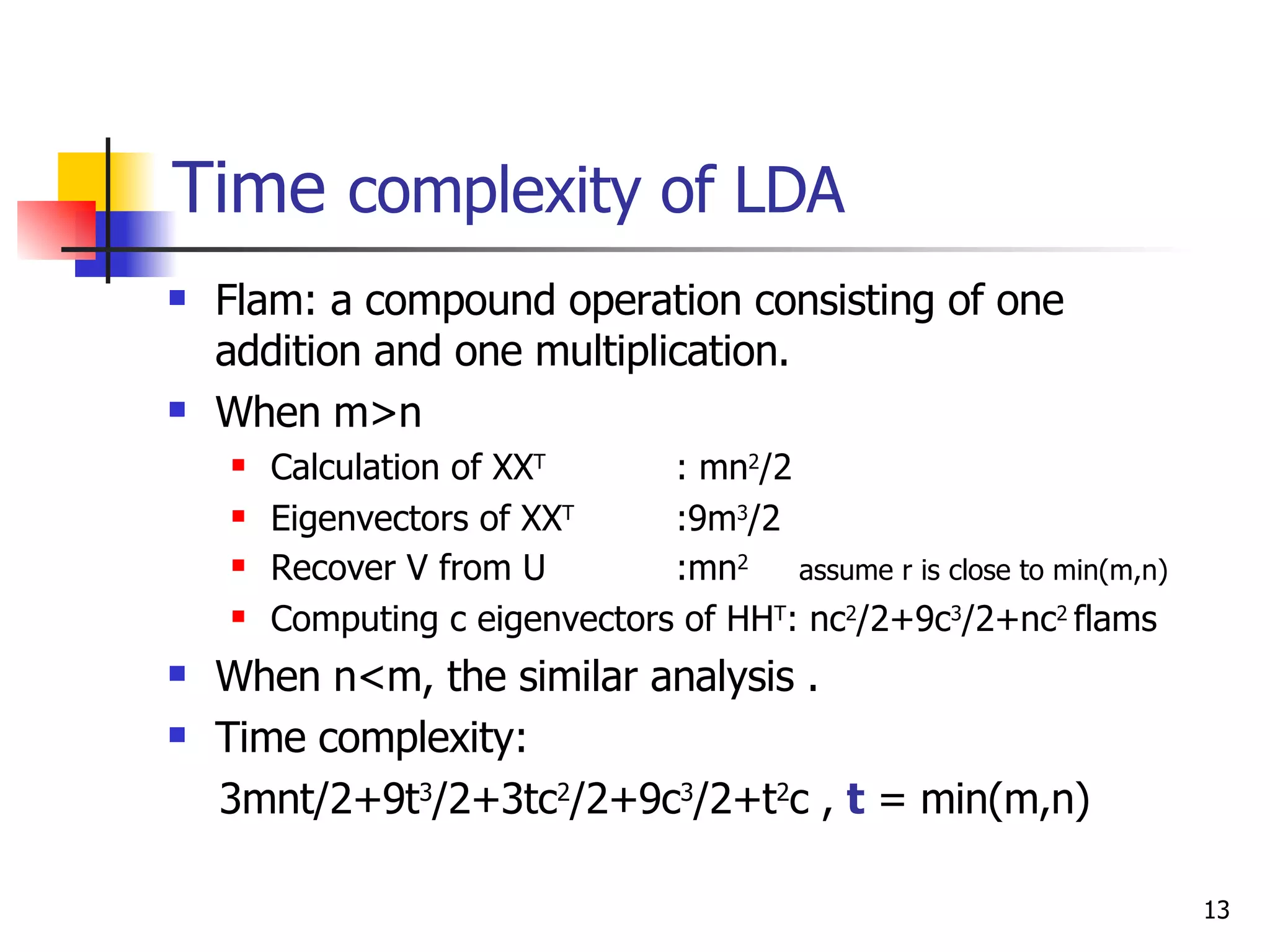
The document proposes a new method called Spectral Regression Discriminant Analysis (SRDA) to address the computational challenges of Linear Discriminant Analysis (LDA) on large, high-dimensional datasets. SRDA combines spectral graph analysis and regression to reduce the time complexity of LDA from quadratic to linear. It works by using the eigenvectors of the within-class scatter matrix to define a regression problem, the solution of which provides the projection vectors that maximize class separability. Experiments on four datasets show SRDA has comparable classification accuracy to LDA but can scale to much larger problems.

1. Training Linear Discriminant Analysis in Linear Time Deng Cai, Xiaofei He, Jiawei Han Reporter : Wei-Ching He 2007/8/23

2. Outline Introduction Linear Discriminant Analysis Spectral Regression Discriminant Analysis Experiment Conclusion

3. Introduction Dimensionality reduction has been a key problem in many field of information procession due to “ curse of dimensionality ”. One of most popular dimensionality reduction algorithm is Linear Discriminant Analysis (LDA)

4. Introduction LDA preserve class separability . LDA involves dense matrices eigen-decomposition which can be expensive both in time and memory. It is infeasible to apply LDA on large scale high dimensional data. Spectral Regression Discriminant Analysis (SRDA) is developed from LDA but has significant computational advantage.

5. Introduction SRDA combines spectral graph analysis and regression. It can be easily scaled to very large high dimensional data sets.

6. Linear Discriminant Analysis (LDA) The objective function of LDA as Eqn (1). Given a set of m smaples x 1 , x 2 ,…,x m belong to c classes. between-class scatter matrix within-class scatter matrix Where μ is total mean vector, m k is number of sample in the k -th class, μ (k) is the average vector of k -th class, and x i (k) is the i - th sample in the k -th class.

7. Linear Discriminant Analysis Define S t =Σ = ( x i – μ ) ( x i – μ ) T as the total scatter matrix and we have S t = S b + S w . So, Eqn. (1) is equivalent to Those optimal a ’s are the eigenvectors corresponding to the non-zero eigenvalue of the generalized eigenvalues Since the rank ( S b ) ≦ c -1, there’re most c -1 eigen-vectors corresponding to non-zero eigenvalues.

8. Computational Analysis of LDA Let x i = x i – μ denote to the centered data point and X (k) = [ x 1 (k) ,…, x m k (k) ] denote to the centered data matrix of k -th class. W (k) is a m k x m k matrix with all elements equal to 1/ m k .

9. Computational Analysis of LDA Then Eqn(5) => Define

10. Computational Analysis of LDA After calculating b ’s, the a ’s can obtained by a=UΣ -1 b Suppose rank( )=r, where U T U = V T V = I , Σ =diag(σ 1 ,σ 2 , …,σ r ) σ 1 ≧σ 2 ≧ …≧σ r ≧0 .

11. 3 steps of LDA 1. SVD decomposition of X to get U , V ,and Σ . 2. Computing b ’s, the eigenvectors of V T WV . 3. Computing a = UΣ -1 b .

12. Linear Discriminant Analysis The left or right singular vectors of X (comun vectors of U or V) are eigenvectors of XX T or X T X . Given U or V, we can recover the other via XV = UΣ or U T X =ΣV T . Eg. In most case, r is close to min(m,n) . So r >>c Computing the eigenvectors of H T H then recover the eigenvectors of HH T is faster than computing the eigenvectors of HH T .

13. Time complexity of LDA Flam: a compound operation consisting of one addition and one multiplication. When m>n Calculation of XX T : mn 2 /2 Eigenvectors of XX T :9m 3 /2 Recover V from U :mn 2 assume r is close to min(m,n) Computing c eigenvectors of HH T : nc 2 /2+9c 3 /2+nc 2 flams When n<m, the similar analysis . Time complexity: 3mnt/2+9t 3 /2+3tc 2 /2+9c 3 /2+t 2 c , t = min(m,n)

14. Spectral Regression Discriminant Analysis (SRDA) Theorem 1. Let y be the eigenvector of W such that Wy = λy . If X T a = y , then a is eigenvector of eigen-problem in Eqn(8). Pf. XWX T a = XWy = X λy =λXX T a .

15. SRDA By theorem 1 , LDA can be obtained through two steps: 1. Solve the eigen-problem in Eqn(12)to get y . 2. Find a which satisfies X T a = y . In reality, such a may not exist. A possible way is to find a which can best fit the equation in the least squares sense: where y i is the i -th element of y

16. Ridge regression If n > m , there’re infinite solutions in Eqn (13). The most popular way to solve this problem is to impose a penalty on the norm of a . Where α ≧0 is a parameter to control the amount of shrinkage.

17. Spectral analysis W is block-diagonal, thus, its eigenvalues and eigenvectors are union of eigen-values and eigenvectors of its blocks. W (k) has only one nonzero eigenvector e (k) Thus, there’re exactly c eigenvector of W with eigen value 1. These eigenvectors of W are

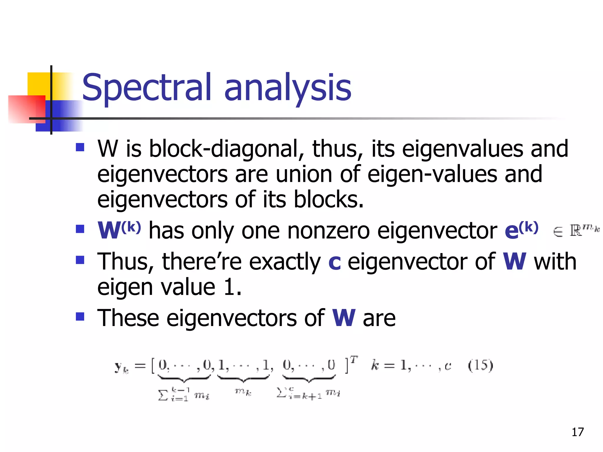
18. Spectral analysis In order to guarantee there exists a vector a which satisfies the linear equation system X T a = y , y should be in the space spanned by the row vectors of X . Since Xe = 0, e =[1,…,1] T is orthogonal to this space. e is in the space of { y k }. We pick e as the first eigenvector of and use Gram-Schmidt process to orthogonzlize the remaining eigenvectors. Remove e , which leave us exactly c -1 eigenvectors of W as below.

19. SRDA in the following discussions, y is one of the eigenvector in Eqn.(16). Eqn.(14) can be rewritten in matrix form as: Respect to a vanish, we get ??

20. Theoretical Analysis Thmeorem 2. If y is in the space spanned by row vectors of X , the corresponding projective function a calculated in SRDA will be the eigenvector of eigen-problem in Eqn.(8) as α deceases to zero. Therefor, a will be one of the projective function of LDA. Corollary 3 If the sample vectors are linearly independent, then all c -1 projective functions in SRDA will be identical to those of LDA as α deceases to zero .

21. Theoretical Analysis The i -th and j -th entries of any vector y in the space spanned by { y k } in Eqn.(15) are the same as long as x i and x j belong to the same class. Thus the i -th and j -th rows of Y are the same, where Y = [ y 1 ,…, y c-1 ] . Corollary (3) shows that when sample is linearly independent, the c -1 projective functions of LDA are exactly the solutions of the c -1 linear equations systems X T a k = y K .

22. Theoretical Analysis Let A = [ a 1 ,…, a c-1 ] be the LDA transformation matrix which embeds the data points into the LDA subspace as: A T X = A T (X + μe T )=Y T + A T μe T The projective functions are usually overfit the traning set thus may not be able to perform well for the test samples, thus the regularization is necessary.

23. Computational Complexity Analysis Two steps Responses generation (by Gram-Schmidt method) mc 2 - c 3 /3 flam and mc+c2 memory Regularized least squares (2 method) Solving normal equations Iterative solution with LSQR

24. Computational Complexity Analysis

25. Experiment Four datasets are used in our experimental study, including face, handwritten digit, spoken letter, and text databases.

26. Experiment (compared algorithms) 1. Linear Discriminant Analysis (LDA). Solving the singularity problem by using SVD . 2. Regularized LDA (RLDA) . Solving the singularity problem by adding some constant values to the diagonal elements of S w , as S w + αI, for some α > 0 and I is an identity matrix. 3. Spectral Regression Discriminant Analysis (SRDA), our approach proposed in this paper. 4. IDR/QR , a LDA variation in which QR decom- position is applied rather than SVD. Thus, IDR/QR is very efficient.

27. Experiment

28. Experiment

29. Parameter selection for SRDA

30. Conclusion SRDA provides an efficient and effective approach for discriminant analysis. SRDA is first one which can handlevery large scale high dimensional data for discriminant analysis.