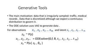
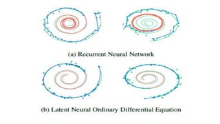
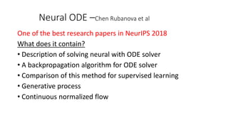
The document provides an overview of Neural ODEs, highlighting their significance in deep learning and referencing key research from NeurIPS 2018. It explains the basics of ordinary differential equations (ODE), their applications, and how they can be used to solve neural network problems, including methods like the adjoint method for backpropagation. Additionally, it discusses continuous normalizing flows and the potential of Neural ODEs in modeling data that is irregularly sampled.

1. Neural ODE
Natan Katz
Natan.katz@gmail.com

2. Lecture’s Summary
• Why do we care about ODE?
• What is ODE?
• Neural ODE –History
• Neural ODE –NeurIPS paper

3. Why do we care?
• NeurIPS 2018 research papers competition
• 4500 papers have been submitted
• One of the best 4 :
Neural ODE (Qi Chen ,Rubanova, Bettencourt ,Duvenaud)
An new usage of both mathematical tool an approach in DL
1. Observing a network as a continuous entity
2. Observing hidden layer as a time function rather a set of
discrete entities

4. What are Differential Equations?
• Equations that has the form
F(X,C) =0
C is a constants vector (e.g. weights).
F is a function.. “generously differentiable”
(until now it is as complicated as a quadratic equation..)
X is a the variable of F and it contains derivatives..
Derivatives of what??!!

5. Classes of Differential Equations
1 Autonomous ODE - 𝑥 =f(x)
2 Non-Autonomous ODE 𝑥 =f(x,t)
3 PDE
𝜕𝑢
𝜕𝑥
+
𝜕𝑢
𝜕𝑡
−
𝜕2 𝑢
𝜕𝑥2 -g(x) = 0
4 SDE 𝑥 =f(x) +𝑑𝑊

6. PDE –Real Life Example
Poisson Equation ∆u =f
u is the potential of a vector field and f is the “source function”
(density or electrical charge)
Burger Equation :
𝜕𝑢
𝜕𝑡
+u
𝜕𝑢
𝜕𝑥
=μ
𝜕2 𝑢
𝜕𝑥2 u is fluid velocity ,
μ the diffusion term, For μ=0 it is used often in shock waves.
and the coolest girl in the hood Navier-Stokes
𝜕𝑈
𝜕𝑡
+ u ∙ 𝛻u =-
𝛻𝑝
𝜌
- μ ∆u +f(x, t) u is fluid velocity

7. Example: Black & Scholes
Stock price:
𝑑S = μS𝑑t +σS𝑑W
Derivative price (using Ito’s lemma):
𝑑V=(μS
𝜕𝑉
𝜕𝑆
+
𝜕𝑉
𝜕𝑡
+
1
2
σ2
S2 𝑑2 𝑉
𝑑2 𝑆
)dt + σS
𝜕𝑉
𝜕𝑆
dW
We wish to have a portfolio with 1 derivative (option ) and 𝛿 stocks
P =V+ 𝛿S
𝑑P =(μS
𝜕𝑉
𝜕𝑆
+
𝜕𝑉
𝜕𝑡
+
1
2
σ2
S2 𝑑2 𝑉
𝑑2 𝑆
+ 𝛿 μS)dt +(σS
𝜕𝑉
𝜕𝑆
+ 𝛿 σS) dW

8. Black & Scholes
Let’s get rid of the randomness
𝛿 =−
𝜕𝑉
𝜕𝑆
We assume no arbitrages (namely we can put it in the bank with risk free r)
Π = -V + S
𝜕𝑉
𝜕𝑆
=> rP𝑑t=𝑑P
Which leads to the PDE
𝜕𝑉
𝜕𝑡
+
1
2
σ2
S2 𝑑2 𝑣
𝑑2 𝑆
+rS
𝜕𝑉
𝜕𝑆
-rV=0

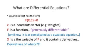
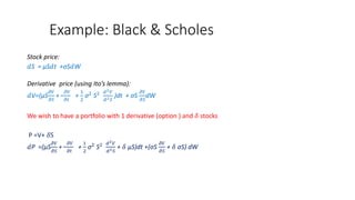
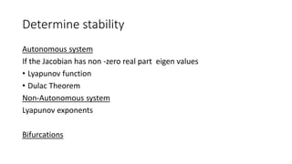
9. ODE –Basic Terminology
𝑥 =f(x) or 𝑥 =f(x,t)
Initial condition
Let the eq. 𝑥 =f(x) we add the initial condition x[0] =c
Example:
𝑥=x by integrating both sides we get
x[t] =𝑒 𝑡
a . We need the i.c. to determine a

10. ODE –Basic Terminology
• ODE solutions never intersect
• For most cases we cannot solve the equation analytically
We aim to study flow patterns in the state space
Ω Limit –the set of points in which flows may converge as time goes to
infinity
α Limit –the set of points in which flows may converge as time goes to minus
infinity
• Elements that we may find :fixed points, closed curves
strange attractors

11. ODE -Terminology
Attractors
A point or compact set in which attracts every i.c.
Fixed Point
F(x)=0 Namely the point that the flow “rests”
Stability
F.p. is stable if the flow does not leave a ε-neighborhood. (homoclinic)

13. Determine stability
Autonomous system
If the Jacobian has non -zero real part eigen values
• Lyapunov function
• Dulac Theorem
Non-Autonomous system
Lyapunov exponents
Bifurcations

14. Further Reading
• Non Autonomous DS, Kloeden & Rasmussen
• ODE - Jack Hale
• Navier Stokes –several books, papers of Edriss Titti
• Theory & applications of SDE –Zeev Schuss
• Books on Heat equation

15. DE & DL
• Consider Resnet
Every layer t satisfies :
ℎ 𝑡+1 =δt f(ℎ 𝑡 θ) + ℎ 𝑡
Haber & Ruthotto (2017) ,Yiping Lu ,Zhong
For infinitesimal time step (nearly continuity) We obtain:
ℎ = f(h, θ)

16. What does it mean?

18. Neural ODE –Chen Rubanova et al
One of the best research papers in NeurIPS 2018
What does it contain?
• Description of solving neural with ODE solver
• A backpropagation algorithm for ODE solver
• Comparison of this method for supervised learning
• Generative process
• Continuous normalized flow

19. A backpropagation algorithm for ODE solver
• There are several methods to solve ODEs such as Euler and
Runge-Kutta , their main difficulties is the amount of
gradients needed
Adjoint Method
min
θ
𝐹 F(z,θ) = 0
𝑇
𝑓 𝑧, 𝑡, θ 𝑑𝑡
g(x(0), θ) = 0
h(x, 𝑥, 𝑡, θ) =0
Note : g,h define together an initial condition problem

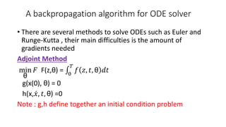
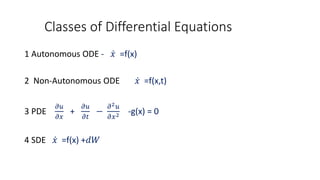
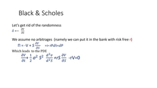
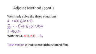
20. Adjoint Method (cont.)
So what do they do in the paper?
𝑧 =f(z,t,θ)
We assume a loss L s.t.
L(z(T) =L[z (0) + 0
𝑇
𝑓 𝑧, 𝑡, θ 𝑑𝑡] -ODE solver friendly 
We define
a(T) =
𝜕𝐿
𝜕𝑧(𝑇)
What is actually z(T)?

22. Adjoint Method (cont.)
We simply solve the three equations:
𝑎 = a(T) 𝑓𝑍 𝑧, 𝑡, θ
𝜕𝐿
𝜕θ
= - 𝑡
0
𝑎(𝑡)𝑓θ 𝑧, 𝑡, θ 𝑑𝑡
𝑧 =f(z,t,θ)
With the i.c. a(T), z(T) , θ0
Torch version github.com/rtqichen/torchdiffeq.

23. Comparison of this method for
supervised learning
They compared on MNIST:
1. Resnet
2. ODE
3. Runge-Kutta
The error is nearly similar where ResNet uses more params.
(ODE –net has about the same as a single layer with 300 units
of Resnet)

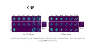
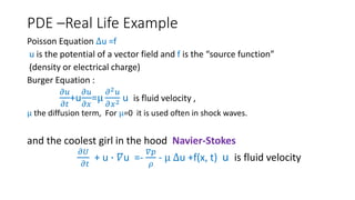
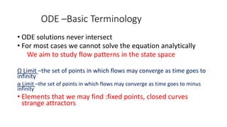
24. Continuous Normalization Flow- CNF
• A method that maps a generic distribution (Gaussianexponents)
Into a more complicate distributions through a sequence of maps
𝑓1 , 𝑓2 , 𝑓3 .…. 𝑓𝑘
The main difficulties here are:
𝑧1= 𝑓(𝑧0 ) => log 𝑝(𝑧1)=log 𝑝(𝑧0) -log det(𝑓𝑍[𝑧0])
Calculating determinants is “costly”.

25. CNF
ODE –solution:
We assume a continuous sequence of maps:
𝜕 log 𝑝( 𝑧 𝑡)
𝜕𝑡
= -tr(𝑓𝑍(t) )
Traces are easier to calculate and linear which allow us to
measure summation of fumctions as well

26. CNF

27. Generative Tools
• The main motivation: data that is irregularly sampled: traffic, medical
records . Data that is discretized although we expect a continuous
distribution to govern it.
• The ODE solution uses VAE to generate data .
For observations 𝑥1 , 𝑥2 , 𝑥3 … 𝑥 𝑚 and latent 𝑧1 , 𝑧2 , 𝑧3 … z 𝑚
𝑧0 ~ P(z)
𝑧1 , 𝑧2 , 𝑧3.. = ODEsolver(0,f, θ, 𝑡1 , 𝑡2 , 𝑡3 … t 𝑚)
𝑥𝑡 ~ P(x| 𝑧𝑡 , θ 𝑥 )

28. Generative ( cont)
In more details:
1. Put 𝑥1 , 𝑥2 , 𝑥3 … 𝑥 𝑚 to RNN
2. Calculate dist params 𝝀 from its hidden states (e.g. mean & std)
3. Sample 𝑧0 from q(𝑧0|𝝀. 𝑥1 , 𝑥2 , 𝑥3)
4. Run ODE solver with 𝑧0 and construct trajectory until 𝑡 𝑘
5. Decode 𝑥′
P(𝑥′
|𝑧𝑡 𝑘
, θ 𝑥)
6. Calculate KL divergence
Log(P(𝑥′
|𝑧𝑡 𝑘
, θ 𝑥)) +log(p(𝒛 𝟎)) –log(q(𝑧0|𝝀. 𝑥1 , 𝑥2 , 𝑥3))
p(𝒛 𝟎) ~N(0,1)

30. Thanks!!!