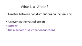
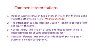
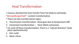
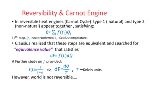
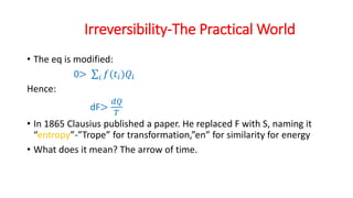
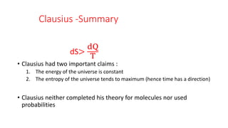
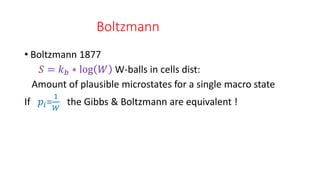
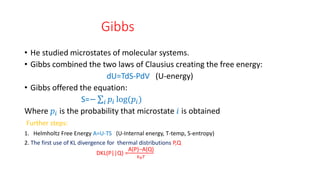
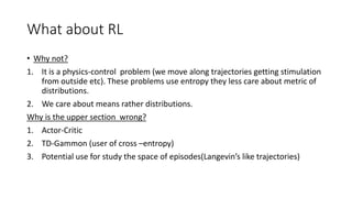
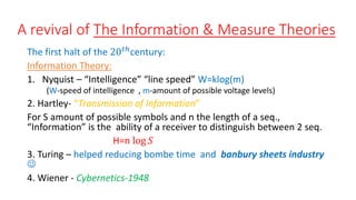
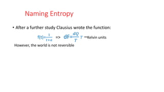
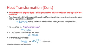
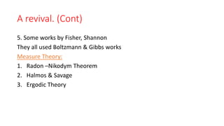
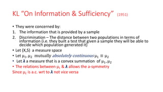
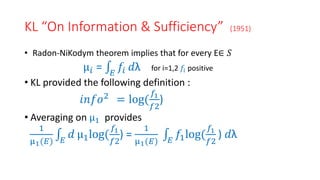
The document discusses KL divergence and related concepts from physics, information theory, and statistics. It covers: 1. The origins of KL divergence in physics from the works of Clausius, Boltzmann, and Gibbs on entropy and thermal distributions. 2. The revival of information theory in the 1950s by Kullback and Leibler, who defined KL divergence as a measure of discrimination between probability distributions. 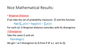3. The connections between KL divergence and other mathematical concepts like Bregman divergence and f-divergence, as well as applications in statistics like Fisher information.

1. KL-Divergence
Relative Entropy

2. What is all About?
• A metric between two distributions on the same r.v.
• A clever Mathematical use of:
• Entropy
• The manifold of distribution functions.

3. Common Interpretations
1. Delta of surprise between two players one think that the true dist is
P and the other thinks it is Q (Wiener, Shannon)
2. The information gain by replacing Q with P (similar to decision trees
not exactly the same)
3. Coding theory- The amount of extra bits needed when going to
code optimized for Q using code optimized for P
4. Bayesian Inference- The amount of information that we gain in
posterior P compared to prior Q

4. KL-Divergence
• Let X r.v. P,Q discrete distributions on X
KL(P||Q) = 𝑥∈X 𝑃 𝑥 ∗ log
𝑃(𝑥)
𝑄(𝑥)
Properties :
1. For P≠ 𝑄 KL(P||Q) is positive. (the magic of Jensen’s ineq.)
2. Non-Symmetric (Symmetry is achieved by KL(P||Q) + KL(Q||P):
It is a subjective metric :it measures the distance as P “understands” it.
3 Continuous case ( here 𝑝 𝑞 are pdfs)
𝐾𝐿(𝑃| 𝑄 = 𝑝(𝑥) 𝑙𝑜𝑔
𝑝(𝑥)
𝑞(𝑥)
dx

5. Let’s re write it :
• Recall
KL(P||Q) = 𝑥∈X 𝑃 𝑥 ∗ log
𝑃(𝑥)
𝑄(𝑥)
=
𝑥∈X 𝑃 𝑥 ∗ log 𝑃 𝑥 - 𝑥∈X 𝑃 𝑥 ∗ log Q(x) = H(P) -Cross Entropy

6. What do we have then?
1. Good Connectivity to physics -the best algo-pusher
(Ask EE, Biometrics and financial-engineering)
2. A coherent foundation process (“Lecturable”)
3. Similarity with known mathematical tools
4. Closely related to well known ML tools

7. ENTROPY

8. Thermo- Dynamics
• Clausius (1850)
• First Law: Energy is preserved–Great!
• A book that falls on the ground, ice cubes
• Clausius (1854)
• Second Law: Heat cannot be transferred from colder to a warmer body
without additional changes. Impressive ! What does it mean ?

9. Heat Transformation
• Clausius denoted the heat transfer from hot body to cold body:
“Verwandlungsinhalt” –content transformation
• There are two transformation types:
1. Transmission transformation –Heat goes due to temperature diff.
2. Conversion transformation – Heat Work conversion
• For each of these transformations there is a “natural direction” (take
place spontaneously):
1. Hot->cold
2. Work->Heat

10. Reversibility & Carnot Engine
• In reversible heat engines (Carnot Cycle) type 1 ( natural) and type 2
(non-natural) appear together , satisfying:
0= 𝑖 𝑓(𝑡𝑖)𝑄𝑖
i-𝑖𝑡ℎ
step, 𝑄𝑖 -heat transferred, 𝑡𝑖 -Celcius temperature.
• Clausius realized that these steps are equivalent and searched for
“equivalence value” that satisfies
dF= 𝑓(𝑡)𝑑𝑄
A Further study on 𝑓 provided:
f(t)=
1
𝑡+𝑎
=> dF=
𝑑𝑄
𝑇
, 𝑇 –Kelvin units
However, world is not reversible….

11. Irreversibility-The Practical World
• The eq is modified:
0> 𝑖 𝑓(𝑡𝑖)𝑄𝑖
Hence:
dF>
𝑑𝑄
𝑇
• In 1865 Clausius published a paper. He replaced F with S, naming it
“entropy”-”Trope” for transformation,”en” for similarity for energy
• What does it mean? The arrow of time.

12. Clausius -Summary
dS>
dQ
T
• Clausius had two important claims :
1. The energy of the universe is constant
2. The entropy of the universe tends to maximum (hence time has a direction)
• Clausius neither completed his theory for molecules nor used
probabilities

13. Boltzmann
• Boltzmann 1877
𝑆 = 𝑘𝑏 ∗ log 𝑊 W-balls in cells dist:
Amount of plausible microstates for a single macro state
If 𝑝𝑖=
1
𝑊
the Gibbs & Boltzmann are equivalent !

14. Gibbs
• He studied microstates of molecular systems.
• Gibbs combined the two laws of Clausius creating the free energy:
dU=TdS-PdV (U-energy)
• Gibbs offered the equation:
S=− 𝑖 𝑝𝑖 log(𝑝𝑖)
Where 𝑝𝑖 is the probability that microstate 𝑖 is obtained
Further steps:
1. Helmholtz Free Energy A=U-TS (U-Internal energy, T-temp, S-entropy)
2. The first use of KL divergence for thermal distributions P,Q
DKL(P||Q) =
A(P)−A(Q)
𝑘𝑏𝑇

15. Data Science Perspective
• We differentiate between two types of variables:
1. Orderable – Numbers ,continuous metric we can say about each
pair of elements who is bigger and to estimate the delta. We have
many quantitative tools.
2. Non-orderable – Categorical, text we cannot compare elements, the
topology is discrete and we hardly have tools.
• Most of us suffered once from “type 2 aversion”

16. Data Science Perspective
• All the three physicists approached their problem with prior
assumption that their data is non-orderable .
• Clausius used prior empirical observation to define order
(temperature) and overcame dealing with such variable
• Gibbs and Boltzmann found a method to assess this space while it is
still non-orderable
• Analogy to reinforcement –the states of episodes

17. Points for further pondering
1. If all the state spaces were orderable, would we care about entropy
(we=those among us that their name is not Clausius)
2. Probability spaces are API for us to use categorical variables
quantitatively

18. Kullback & Leibler

19. A revival of The Information & Measure Theories
The first halt of the 20𝑡ℎ
century:
Information Theory:
1. Nyquist – “Intelligence” “line speed” W=klog(m)
(W-speed of intelligence , m-amount of possible voltage levels)
2. Hartley- “Transmission of Information”
For S amount of possible symbols and n the length of a seq.,
“Information” is the ability of a receiver to distinguish between 2 seq.
H=n log 𝑆
3. Turing – helped reducing bombe time and banbury sheets industry

4. Wiener - Cybernetics-1948

20. A revival. (Cont)
5. Some works by Fisher, Shannon
They all used Boltzmann & Gibbs works
Measure Theory:
1. Radon –Nikodym Theorem
2. Halmos & Savage
3. Ergodic Theory

21. KL “On Information & Sufficiency” (1951)
• They were concerned by:
1. The information that is provided by a sample
2. Discrimination – The distance between two populations in terms of
information (i.e. they built a test that given a sample they will be able to
decide which population generated it)
• Let (X,S) a measure space
• Let μ1, μ2 mutually absolutely continuous μ1 ≡ μ2
• Let λ a measure that is a convex summation of μ1, μ2
• The relations between μ𝑖 & λ allows the a-symmetry
Since μ𝑖 is a.c. wrt to λ not vice versa

22. KL “On Information & Sufficiency” (1951)
• Radon-NiKodym theorem implies that for every E∈ 𝑆
μ𝑖 = 𝐸
𝑓𝑖 𝑑λ for i=1,2 𝑓𝑖 positive
• KL provided the following definition :
𝑖𝑛𝑓𝑜2
= log(
𝑓1
𝑓2
)
• Averaging on μ1 provides
1
μ1(𝐸) 𝐸
𝑑 μ1log(
𝑓1
𝑓2
) =
1
μ1(𝐸) 𝐸
𝑓1log(
𝑓1
𝑓2
) 𝑑λ

23. Let’s stop and summarizes
• Connection to physics –Yes
• Foundation process - Yes
• What about Math and ML?

24. Nice Mathematical Results:
• Bregman Distance
If we take the set of probability measures Ω and the function
F(p)= 𝑥 𝑝 𝑥 ∗ log(𝑝 𝑥 − 𝑝(𝑥)
For each q∈ Ω Bregman distance coincides with KL-divergence
f-Divergence
Take the same Ω and set
F(x)=xlog(𝑥)
We get F as f-divergence to Q from P (P a.c. wrt to Q)

25. Why is this important?
• These metrics are a-symmetric
• Similarity between mathematical result hints about their importance
• It presents potential tools and modifications

26. Shannon & Communication Theory
• A language entropy is defined
H(p)= − 𝑖 𝑝𝑖 log2(𝑝𝑖) -measured in bits
Where 𝑝𝑖 is the weight of the 𝑖𝑡ℎ
𝑙𝑒𝑡𝑡𝑒𝑟
• −𝑙𝑜𝑔2 𝑝𝑖 -The amount of information that a sample brings (how surprise
we are by 𝑝𝑖) Entropy is the average info we may obtain
• I(X,Y)= 𝑋,𝑌 𝑝(𝑋, 𝑌) log
𝑝(𝑋,𝑌)
𝑝 𝑋 𝑝(𝑌)
(For Q(x,y)=P(x)P(Y) it is simply KL)
• The Entropy of a language is the lowest boundary for the average coding
length (Kraft inequality)
• If P,Q dist. And we optimized model upon P KL is the amount of extra bits
we will have to add if we use the code for dist. Q (see the importance of A-
simmetry)

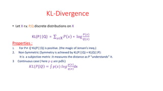
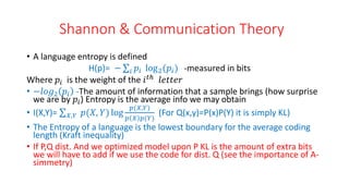
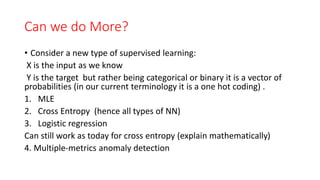
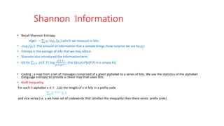
27. Fisher Information
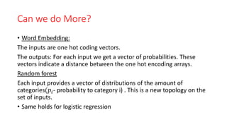
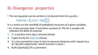
• The idea : f a distribution on space X and parameter θ. We are
interested in the information that X provides on θ .
• Obviously information is gained when θ is not optimal
• It is one of the early uses of log-likelihood in statistics
E[
𝜕 log f(X,θ )
𝜕θ
| θ] = 0
Fisher Information
I(θ) =-E[
𝑑2 log 𝑓(𝑥,θ)
𝑑θ
2 ]= (
𝜕 log f(X,θ )
𝜕θ
)2 f(X,θ )dx

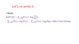
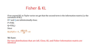
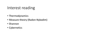
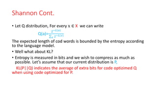
28. Fisher Information
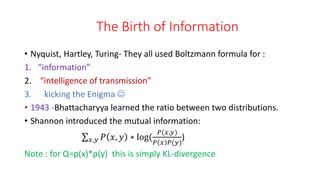
• It can be seen that the information is simply the variance.
• When θ is a vector we get a matrix “Fisher Information matrix” that is used
in differential geometry.
𝒂𝒊𝒋 = E[
𝝏 𝒍𝒐𝒈 f(X,θ )
𝝏θ𝒊
𝝏 𝒍𝒐𝒈 f(X,θ )
𝝏θ𝒋
| θ]
Where Do we use this?
Jeffreys Prior- A method to choose prior distribution in Bayesian inference
P(θ) α 𝑑𝑒𝑡(𝐼( θ))

29. Fisher & KL
If we expand KL to Taylor series we get that the second term is the information matrix (i.e the
curvature of KL).
If P and Q are infinitesimally close:
P=P(θ)
Q=P(θ0)
Since
KL(P||P)= 0 ,
𝜕KL(𝑃(θ)
𝜕θ
=0
We have:
For two distributions that are infi. Close, KL and Fisher Information matrix are
identical

30. PMI-Pointwise Mutual Information
PMI(X=a, Y=b)= log
𝑃(𝑥=𝑎,𝑦=𝑏)
𝑃 𝑥=𝑎 ∗𝑃(𝑦=𝑏)
1. Setting Y to be constant and averaging over all x values we get :
KL(X|| Y=b)
2. This metric is relevant for many commercial tasks such as churn
prediction or digital containment : We compare population in general
to its distribution for a given category
3. PMI is the theoretical solution for factorizing the matrix in word
embedding (Levy & Goldberger (2014) Neural word embedding as
implicit factorization)

31. Real World use
Cross Entropy is commonly used as a loss function in many types of
neural network applications such as ANN, RNN and word embedding as
well ad logistic regression.
• In processes such ad HDP or EM we may use it after
adding topics dividing Gaussian.
• Variational Inference
• Mutual Information
• Log-likelihood (show one item in the summation)

32. What about RL
• Why not?
1. It is a physics-control problem (we move along trajectories getting stimulation
from outside etc). These problems use entropy they less care about metric of
distributions.
2. We care about means rather distributions.
Why is the upper section wrong?
1. Actor-Critic
2. TD-Gammon (user of cross –entropy)
3. Potential use for study the space of episodes(Langevin’s like trajectories)

33. Can we do More?
• Consider a new type of supervised learning:
X is the input as we know
Y is the target but rather being categorical or binary it is a vector of
probabilities (in our current terminology it is a one hot coding) .
1. MLE
2. Cross Entropy (hence all types of NN)
3. Logistic regression
Can still work as today for cross entropy (explain mathematically)
4. Multiple-metrics anomaly detection

34. Interest reading
• Thermodynamics
• Measure theory (Radon-Nykodim)
• Shannon
• Cybernetics

35. End!!!
•Freedom

36. Entropy - Summary
• Most of the state spaces that have described are endowed with
discrete topology that suffers from no natural order (categorical
variables)
• It is difficult to use common analytical tools on such spaces.
• The manifold of probability functions is an API for using categorical
data with analytical tools.
• Note: if all the data in the world was orderable, we might not need
entropy.

37. garbage
• “LEARNING THE DISTRIBUTION WITH LARGEST MEAN: TWO BANDIT FRAMEWORKS” kaufmann Garivier

38. KL-Divergence -properties
• The last equation can be written in its discrete form for p,q dist. :
KL(p||q) = 𝑥 𝑝 𝑥 ∗ log(
𝑝(𝑥)
𝑞(𝑥)
)
It is a metric on the manifold of probability measures of a given variables.
• KL- If one assumes distr. P and other assumes Q. The for a sample x KL
indicates the delta of surprisal
1. KL is positive since log is concave (show)
2. It gets 0 only for KL(p||p) (show)
3. It is not asymmetric since it aims to measure distances with respect to p
(p “decides subjectively” which function is close )
4. KL(P||Q)+KL(Q||P) is symmetric

39. The Birth of Information
• Nyquist, Hartley, Turing- They all used Boltzmann formula for :
1. “information”
2. “intelligence of transmission”
3. kicking the Enigma 
• 1943 -Bhattacharyya learned the ratio between two distributions.
• Shannon introduced the mutual information:
𝑥,𝑦 𝑃 𝑥, 𝑦 ∗ log(
𝑃(𝑥,𝑦)
𝑃 𝑥 𝑃(𝑦)
)
Note : for Q=p(x)*p(y) this is simply KL-divergence

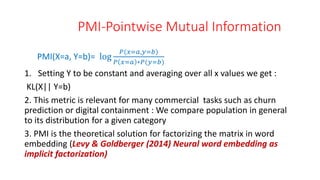
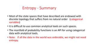
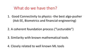
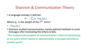
40. Wiener’s Work
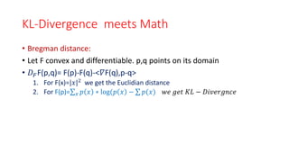
• Cybernetics-1948
• The delta between two distributions:
1. Assume that we draw number and a-priorically we think the
distribution is [0,1] uniform. This number due to set theory can be
written as an infinite series of bits. Let’s assume that a smaller
interval is needed to asses it (a, b)< 0,1
2. We simply need to measure until the first bit that is not 0.
The posterior information is -
log(𝑎,𝑏)
log(0,1)
(explain!!)

41. KL-Divergence meets Math
• Bregman distance:
• Let F convex and differentiable. p,q points on its domain
• 𝐷𝐹F(p,q)= F(p)-F(q)-<𝛻F(q),p-q>
1. For F(x)=|𝑥|2 we get the Euclidian distance
2. For F(p)= 𝑥 𝑝 𝑥 ∗ log(𝑝 𝑥 − 𝑝(𝑥) 𝑤𝑒 𝑔𝑒𝑡 𝐾𝐿 − 𝐷𝑖𝑣𝑒𝑟𝑔𝑛𝑐𝑒

42. KL-Divergence meets Math
• f-divergence
• Ω –measure space ,P,Q measures s.t. P absolutely continuous w.r.t Q
f continuous f(1)=0. The f-divergence from Q to P is :
𝐷𝑓(𝑃||𝑄) = Ω 𝑓
𝑑𝑃
𝑑𝑄
𝑑𝑄
For f(x)=xlog 𝑥 KL is f-divergence.

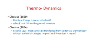
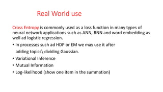
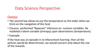
43. Fisher Information- (cont)
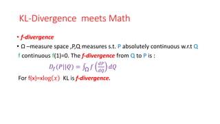
If θ is a vector, I(θ) is a matrix
𝑎𝑖𝑗=E[ (
𝜕 log f(X,θ )
𝜕θ𝑖
)(
𝜕 log f(X,θ )
𝜕θ𝑗
)| θ] –Fisher information metric
Jeffrey’s Prior : P(θ) α 𝑑𝑒𝑡(𝐼( θ))
If P and Q are infinitesimally close:
P=P(θ)
Q=P(θ0)
KL(P||Q)~Fisher information metric :
KL(P||P)=0
𝜕KL(𝑃(θ)
𝜕θ
=0
Hence the leading order of KL near θ is the second order which is the Fisher information metric
(i.e. the Fisher information metric is the second term in Taylor series of KL)

44. Shannon Information
• Recall Shannon Entropy:
H(p)= − 𝑖 𝑝𝑖 𝑙𝑜𝑔2 𝑝𝑖 which we measure in bits
• -𝑙𝑜𝑔2 𝑝𝑖 -The amount of information that a sample brings (how surprise we are by 𝑝𝑖)
• Entropy is the average of info that we may obtain.
• Shannon also introduced the information term:
• I(X,Y)= 𝑋,𝑌 𝑝(𝑋, 𝑌) log
𝑝(𝑋,𝑌)
𝑝 𝑋 𝑝(𝑌)
(For Q(x,y)=P(x)P(Y) it is simply KL)
• Coding : a map from a set of messages comprised of a given alphabet to a series of bits. We use the statistics of the alphabet
(language entropy) to provide a clever map that saves bits.
• Kraft Inequality:
For each X alphabet x ∈ X ,L(x) the length of x in bits in a prefix code
𝑥 2−𝐿(𝑥)
≤ 1
and vice versa (i.e. a we have set of codewords that satisfies this inequality then there exists prefix code) .

45. Shannon & Communication Theory
• A language entropy is defined
H= − 𝑖 𝑝𝑖 log2(𝑝𝑖)
Where 𝑝𝑖 is the weight of the 𝑖𝑡ℎ 𝑙𝑒𝑡𝑡𝑒𝑟
• −𝑙𝑜𝑔2 𝑝𝑖
• Shannon studied communication mainly optimal methods to send
messages after translating the letters to bits.
“The fundamental problem of communication is that of reproducing
at one point either exactly or approximately a message selected at
another point”

46. Shannon Cont.
• Let Q distribution, For every x ∈ X we can write
Q(a)=
2−𝐿(𝑎)
𝑥 2−𝐿(𝑥)
The expected length of cod words is bounded by the entropy according
to the language model.
• Well what about KL?
• Entropy is measured in bits and we wish to compress as much as
possible. Let’s assume that our current distribution is P,
KL(P||Q) indicates the average of extra bits for code optizimed Q
when using code optimized for P.

47. Shannon & Communication Theory
• A language entropy is defined
H= − 𝑖 𝑝𝑖 log2(𝑝𝑖)
Where 𝑝𝑖 is the weight of the 𝑖𝑡ℎ 𝑙𝑒𝑡𝑡𝑒𝑟
• −𝑙𝑜𝑔2 𝑝𝑖
• Shannon studied communication mainly optimal methods to send
messages after translating the letters to bits.
“The fundamental problem of communication is that of reproducing
at one point either exactly or approximately a message selected at
another point”

48. Data Science Perspective
Clausius:
• The second law allows to use the temperature as the order when we
think on the navigation of the heat.
• Clausius performed “Bayesian” inference on numeric variables. He
modeled a latent variable (entropy) upon observations (temperature).
• Example:
If the heat was an episode in re-inforcement learning then all the
policies would be deterministic, we would concern only about the size
of the rewards.

49. Naming Entropy
• After a further study Clausius wrote the function:
f(t)=
1
𝑡+𝑎
=> dF=
𝑑𝑄
𝑇
𝑇 –Kelvin units
However, the world is not reversible

50. Heat Transformation (Cont)
• In real life heat engines type 1 takes place in the natural direction and type 2 in the
unnatural
• Clausius realized that in reversible engines (Carnot engines) these transformations are
nearly equivalent and satisfy
0= 𝑖 𝑓(𝑡𝑖)𝑄𝑖 For 𝑄𝑖 the heat transformed and 𝑡𝑖 Celsius temperature .
• He searched for “equivalence value” :
dF=𝑓(𝑡𝑖)𝑄𝑖
• In continuous terminology we have:
dF= 𝑓(𝑡)𝑑𝑄
A further study provided :
f(t)=
1
𝑡+𝑎
=> dF=
𝑑𝑄
𝑇
𝑇 –Kelvin units
However, world is not reversible….

51. Fisher Information
• Let X r.v. f(X,θ) its density function where θ is a parameter
• It can be shown that :
E[
𝜕 log f(X,θ )
𝜕θ
| θ] = 0
The variance of this derivative is denoted Fisher Information
I(θ) = E[
𝜕 log f(X,θ )
𝜕θ
2
| θ]=
𝜕 log f(X,θ )
𝜕θ
2
f(X,θ )dx
• The idea is to estimate the amount of information that the samples of
X (the observed data) provide on θ

52. Can we do More?
• Word Embedding:
The inputs are one hot coding vectors.
The outputs: For each input we get a vector of probabilities. These
vectors indicate a distance between the one hot encoding arrays.
Random forest
Each input provides a vector of distributions of the amount of
categories(𝑝𝑖- probability to category i) . This is a new topology on the
set of inputs.
• Same holds for logistic regression