Download as PDF, PPTX

![Objective
6
xn
✓
˛ D 1:5; D 1
N
data {
i n t N; // number of observations
i n t x [N ] ; // d i s c r e t e - valued observations
}
parameters {
// l a t e n t variable , must be p o s i t i v e
real < lower=0> theta ;
}
model {
// non - conjugate p r i o r f o r l a t e n t v a r i a b l e
theta ~ weibull ( 1 . 5 , 1) ;
// l i k e l i h o o d
f o r (n in 1:N)
x [ n ] ~ poisson ( theta ) ;
}
Figure 2: Specifying a simple nonconjugate probability model in Stan.
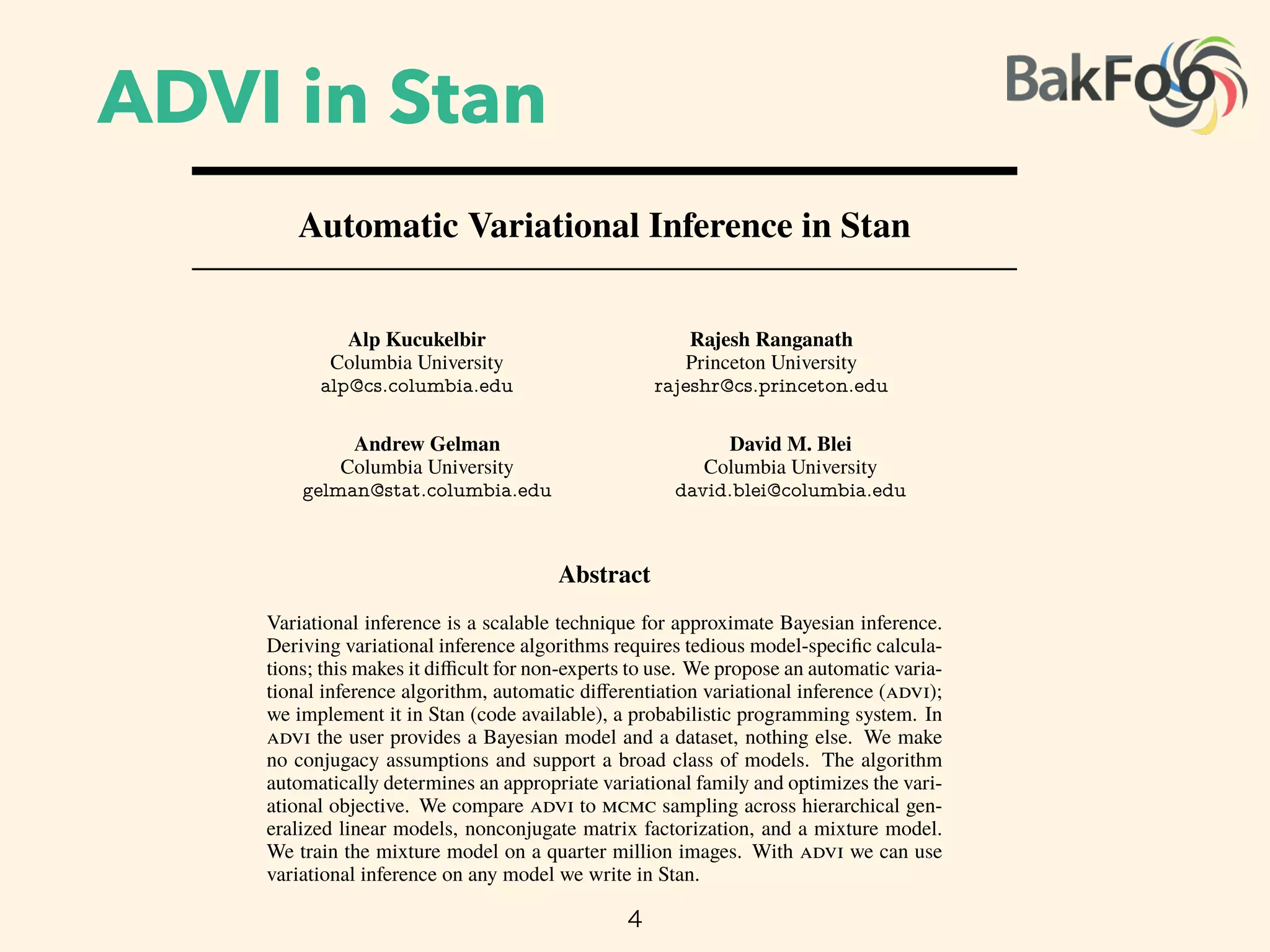
analysis posits a prior density p.✓/ on the latent variables. Combining the likelihood with the prior
gives the joint density p.X; ✓/ D p.X j ✓/ p.✓/.
We focus on approximate inference for di erentiable probability models. These models have contin-
uous latent variables ✓. They also have a gradient of the log-joint with respect to the latent variables
r✓ log p.X; ✓/. The gradient is valid within the support of the prior supp.p.✓// D
˚
✓ j ✓ 2
RK
and p.✓/ > 0 ✓ RK
, where K is the dimension of the latent variable space. This support set
is important: it determines the support of the posterior density and plays a key role later in the paper.
We make no assumptions about conjugacy, either full or conditional.2
For example, consider a model that contains a Poisson likelihood with unknown rate, p.x j ✓/. The
observed variable x is discrete; the latent rate ✓ is continuous and positive. Place a Weibull prior
on ✓, defined over the positive real numbers. The resulting joint density describes a nonconjugate
di erentiable probability model. (See Figure 2.) Its partial derivative @=@✓ p.x; ✓/ is valid within the
support of the Weibull distribution, supp.p.✓// D RC
⇢ R. Because this model is nonconjugate, the
posterior is not a Weibull distribution. This presents a challenge for classical variational inference.
In Section 2.3, we will see how handles this model.
Many machine learning models are di erentiable. For example: linear and logistic regression, matrix
factorization with continuous or discrete measurements, linear dynamical systems, and Gaussian pro-
cesses. Mixture models, hidden Markov models, and topic models have discrete random variables.
Marginalizing out these discrete variables renders these models di erentiable. (We show an example
in Section 3.3.) However, marginalization is not tractable for all models, such as the Ising model,
sigmoid belief networks, and (untruncated) Bayesian nonparametric models.
2.2 Variational Inference
Bayesian inference requires the posterior density p.✓ j X/, which describes how the latent variables
vary when conditioned on a set of observations X. Many posterior densities are intractable because
their normalization constants lack closed forms. Thus, we seek to approximate the posterior.
ADVI
Big
Data
Model](https://image.slidesharecdn.com/nips-yomi2016-01-20-160120081335/75/Automatic-Variational-Inference-in-Stan-NIPS2015_yomi2016-01-20-6-2048.jpg)
![Advantage
• very fast
• able to handle big data
• no hustle
• already available on stan
7
102
103
900
600
300
0
Seconds
AverageLogPredictive
ADVI
NUTS [5]
(a) Subset of 1000 images
102
103
800
400
0
400
Seconds
AverageLogPredictive
B=
B=
B=
B=
(b) Full dataset of 250 000 images
Figure 1: Held-out predictive accuracy results | Gaussian mixture model ( ) of the imag
image histogram dataset. (a) outperforms the no-U-turn sampler ( ), the default sam
method in Stan [5]. (b) scales to large datasets by subsampling minibatches of size B fr
dataset at each iteration [3]. We present more details in Section 3.3 and Appendix J.
Figure 1 illustrates the advantages of our method. Consider a nonconjugate Gaussian mixture
for analyzing natural images; this is 40 lines in Stan (Figure 10). Figure 1a illustrates Ba
inference on 1000 images. The y-axis is held-out likelihood, a measure of model fitness;
Gaussian mixture model (gmm) of the imageCLEF image histogram dataset.](https://image.slidesharecdn.com/nips-yomi2016-01-20-160120081335/75/Automatic-Variational-Inference-in-Stan-NIPS2015_yomi2016-01-20-7-2048.jpg)
![Non-Conjugate
11
xn
✓
˛ D 1:5; D 1
N
data {
i n t N; // number of observations
i n t x [N ] ; // d i s c r e t e - valued observations
}
parameters {
// l a t e n t variable , must be p o s i t i v e
real < lower=0> theta ;
}
model {
// non - conjugate p r i o r f o r l a t e n t v a r i a b l e
theta ~ weibull ( 1 . 5 , 1) ;
// l i k e l i h o o d
f o r (n in 1:N)
x [ n ] ~ poisson ( theta ) ;
}
Figure 2: Specifying a simple nonconjugate probability model in Stan.
nalysis posits a prior density p.✓/ on the latent variables. Combining the likelihood with the pr
ives the joint density p.X; ✓/ D p.X j ✓/ p.✓/.
We focus on approximate inference for di erentiable probability models. These models have cont
ous latent variables ✓. They also have a gradient of the log-joint with respect to the latent variab
@
@✓ p(x, ✓)
is valid within the support of Weibull diatrib.
supp (p(✓)) = R+
⇢ R](https://image.slidesharecdn.com/nips-yomi2016-01-20-160120081335/75/Automatic-Variational-Inference-in-Stan-NIPS2015_yomi2016-01-20-11-2048.jpg)
![Variational Inference
• posterior density: lack closed form
• to approximate the posterior
• find
• VI minimizes the KL divergence of
12
or discrete measurements, linear dynamical systems, and Gaussian pro-
en Markov models, and topic models have discrete random variables.
te variables renders these models di erentiable. (We show an example
rginalization is not tractable for all models, such as the Ising model,
untruncated) Bayesian nonparametric models.
e posterior density p.✓ j X/, which describes how the latent variables
t of observations X. Many posterior densities are intractable because
ack closed forms. Thus, we seek to approximate the posterior.
nsity q.✓ I / parameterized by . We make no assumptions about its
find the parameters of q.✓ I / to best match the posterior according to
l inference ( ) minimizes the Kullback-Leibler ( ) divergence from
rior [2],
⇤
D arg min KL.q.✓ I / k p.✓ j X//: (1)
so lacks a closed form. Instead we maximize the evidence lower bound
rgence,
D Eq.✓/
⇥
log p.X; ✓/
⇤
Eq.✓/
⇥
log q.✓ I /
⇤
:
n of the joint density under the approximation, and the second is the
ity. Maximizing the minimizes the divergence [1, 16].
gate model is in the same family as the prior; a conditionally conjugate model
, we will see how handles this model.
e learning models are di erentiable. For example: linear and logistic regression, matrix
with continuous or discrete measurements, linear dynamical systems, and Gaussian pro-
re models, hidden Markov models, and topic models have discrete random variables.
out these discrete variables renders these models di erentiable. (We show an example
.) However, marginalization is not tractable for all models, such as the Ising model,
f networks, and (untruncated) Bayesian nonparametric models.
nal Inference
ence requires the posterior density p.✓ j X/, which describes how the latent variables
nditioned on a set of observations X. Many posterior densities are intractable because
ation constants lack closed forms. Thus, we seek to approximate the posterior.
pproximating density q.✓ I / parameterized by . We make no assumptions about its
ort. We want to find the parameters of q.✓ I / to best match the posterior according to
ction. Variational inference ( ) minimizes the Kullback-Leibler ( ) divergence from
tion to the posterior [2],
⇤
D arg min KL.q.✓ I / k p.✓ j X//: (1)
divergence also lacks a closed form. Instead we maximize the evidence lower bound
xy to the divergence,
L. / D Eq.✓/
⇥
log p.X; ✓/
⇤
Eq.✓/
⇥
log q.✓ I /
⇤
:
is an expectation of the joint density under the approximation, and the second is the
variational density. Maximizing the minimizes the divergence [1, 16].
or of a fully conjugate model is in the same family as the prior; a conditionally conjugate model
y within the complete conditionals of the model [3].
bution. This presents a challenge for classical variational inference.
handles this model.
are di erentiable. For example: linear and logistic regression, matrix
discrete measurements, linear dynamical systems, and Gaussian pro-
Markov models, and topic models have discrete random variables.
variables renders these models di erentiable. (We show an example
inalization is not tractable for all models, such as the Ising model,
ntruncated) Bayesian nonparametric models.
posterior density p.✓ j X/, which describes how the latent variables
of observations X. Many posterior densities are intractable because
ck closed forms. Thus, we seek to approximate the posterior.
ity q.✓ I / parameterized by . We make no assumptions about its
d the parameters of q.✓ I / to best match the posterior according to
nference ( ) minimizes the Kullback-Leibler ( ) divergence from
or [2],
D arg min KL.q.✓ I / k p.✓ j X//: (1)
lacks a closed form. Instead we maximize the evidence lower bound
gence,
Eq.✓/
⇥
log p.X; ✓/
⇤
Eq.✓/
⇥
log q.✓ I /
⇤
:
of the joint density under the approximation, and the second is the
y. Maximizing the minimizes the divergence [1, 16].
di erentiable probability model. (See Figure 2.) Its partial derivative @=@✓ p.x;
support of the Weibull distribution, supp.p.✓// D RC
⇢ R. Because this mode
posterior is not a Weibull distribution. This presents a challenge for classical v
In Section 2.3, we will see how handles this model.
Many machine learning models are di erentiable. For example: linear and logis
factorization with continuous or discrete measurements, linear dynamical system
cesses. Mixture models, hidden Markov models, and topic models have discre
Marginalizing out these discrete variables renders these models di erentiable. (
in Section 3.3.) However, marginalization is not tractable for all models, such
sigmoid belief networks, and (untruncated) Bayesian nonparametric models.
2.2 Variational Inference
Bayesian inference requires the posterior density p.✓ j X/, which describes how
vary when conditioned on a set of observations X. Many posterior densities ar
their normalization constants lack closed forms. Thus, we seek to approximate
Consider an approximating density q.✓ I / parameterized by . We make no a
shape or support. We want to find the parameters of q.✓ I / to best match the p
some loss function. Variational inference ( ) minimizes the Kullback-Leibler (
the approximation to the posterior [2],
⇤
D arg min KL.q.✓ I / k p.✓ j X//:
Typically the divergence also lacks a closed form. Instead we maximize the e
( ), a proxy to the divergence,
L. / D E
⇥
log p.X; ✓/
⇤
E
⇥
log q.✓ I /
⇤
:
iable probability model. (See Figure 2.) Its partial derivative @=@✓ p.x; ✓/ is valid within the
of the Weibull distribution, supp.p.✓// D RC
⇢ R. Because this model is nonconjugate, the
is not a Weibull distribution. This presents a challenge for classical variational inference.
n 2.3, we will see how handles this model.
achine learning models are di erentiable. For example: linear and logistic regression, matrix
tion with continuous or discrete measurements, linear dynamical systems, and Gaussian pro-
Mixture models, hidden Markov models, and topic models have discrete random variables.
lizing out these discrete variables renders these models di erentiable. (We show an example
n 3.3.) However, marginalization is not tractable for all models, such as the Ising model,
belief networks, and (untruncated) Bayesian nonparametric models.
riational Inference
inference requires the posterior density p.✓ j X/, which describes how the latent variables
en conditioned on a set of observations X. Many posterior densities are intractable because
malization constants lack closed forms. Thus, we seek to approximate the posterior.
an approximating density q.✓ I / parameterized by . We make no assumptions about its
support. We want to find the parameters of q.✓ I / to best match the posterior according to
s function. Variational inference ( ) minimizes the Kullback-Leibler ( ) divergence from
oximation to the posterior [2],
⇤
D arg min KL.q.✓ I / k p.✓ j X//: (1)
y the divergence also lacks a closed form. Instead we maximize the evidence lower bound
a proxy to the divergence,
L. / D Eq.✓/
⇥
log p.X; ✓/
⇤
Eq.✓/
⇥
log q.✓ I /
⇤
:](https://image.slidesharecdn.com/nips-yomi2016-01-20-160120081335/75/Automatic-Variational-Inference-in-Stan-NIPS2015_yomi2016-01-20-12-2048.jpg)
![Variational Inference
• KL divergence lacks of closed form
• maximize the evidence lower bound (ELBO)
• VI is difficult to automate
• non-conjugate
• blab-box, fixed v approx.
13
when conditioned on a set of observations X. Many posterior densities are intractable because
normalization constants lack closed forms. Thus, we seek to approximate the posterior.
sider an approximating density q.✓ I / parameterized by . We make no assumptions about its
e or support. We want to find the parameters of q.✓ I / to best match the posterior according to
e loss function. Variational inference ( ) minimizes the Kullback-Leibler ( ) divergence from
pproximation to the posterior [2],
⇤
D arg min KL.q.✓ I / k p.✓ j X//: (1)
cally the divergence also lacks a closed form. Instead we maximize the evidence lower bound
), a proxy to the divergence,
L. / D Eq.✓/
⇥
log p.X; ✓/
⇤
Eq.✓/
⇥
log q.✓ I /
⇤
:
first term is an expectation of the joint density under the approximation, and the second is the
opy of the variational density. Maximizing the minimizes the divergence [1, 16].
The posterior of a fully conjugate model is in the same family as the prior; a conditionally conjugate model
his property within the complete conditionals of the model [3].
3
The minimization problem from Eq. (1) becomes
⇤
D arg max L. / such that supp.q.✓ I // ✓ supp.p.✓ j X//: (2)
We explicitly specify the support-matching constraint implied in the divergence.3
We highlight
this constraint, as we do not specify the form of the variational approximation; thus we must ensure
that q.✓ I / stays within the support of the posterior, which is defined by the support of the prior.
Why is di cult to automate? In classical variational inference, we typically design a condition-
ally conjugate model. Then the optimal approximating family matches the prior. This satisfies the
support constraint by definition [16]. When we want to approximate models that are not condition-
ally conjugate, we carefully study the model and design custom approximations. These depend on
the model and on the choice of the approximating density.
One way to automate is to use black-box variational inference [8, 9]. If we select a density whose
support matches the posterior, then we can directly maximize the using Monte Carlo ( )
integration and stochastic optimization. Another strategy is to restrict the class of models and use a](https://image.slidesharecdn.com/nips-yomi2016-01-20-160120081335/75/Automatic-Variational-Inference-in-Stan-NIPS2015_yomi2016-01-20-13-2048.jpg)
![Transformation apch
• support of latent var > real space
• transformed joint density(Appendix D)
• example:
16
oach. First we automatically transform the support of the latent
inate space. Then we posit a Gaussian variational density. The
n approximation in the original variable space and guarantees
osterior. Here is how it works.
Constrained Variables
he latent variables ✓ such that they live in the real coordinate
rentiable function T W supp.p.✓// ! RK
and identify the
he transformed joint density g.X; ⇣/ is
D p X; T 1
.⇣/
ˇ
ˇ det JT 1 .⇣/
ˇ
ˇ;
iginal latent variable space, and JT 1 is the Jacobian of the
nuous probability densities require a Jacobian; it accounts for
umes [17]. (See Appendix D.)
The rate ✓ lives in RC
. The logarithm ⇣ D T .✓/ D log.✓/
s Jacobian adjustment is the derivative of the inverse of the
e transformed density is
x j exp.⇣// Weibull.exp.⇣/ I 1:5; 1/ exp.⇣/:
mation.
implement our algorithm in Stan to enable generic inference.
t automatically handles transformations. It works by applying
corresponding Jacobians to the joint model density.4
This
variables in our model to the real coordinate space. Then we posit a G
transformation induces a non-Gaussian approximation in the origina
that it stays within the support of the posterior. Here is how it works
2.3 Automatic Transformation of Constrained Variables
Begin by transforming the support of the latent variables ✓ such that
space RK
. Define a one-to-one di erentiable function T W supp.p
transformed variables as ⇣ D T .✓/. The transformed joint density g
g.X; ⇣/ D p X; T 1
.⇣/
ˇ
ˇ det JT 1 .⇣/
where p is the joint density in the original latent variable space, a
inverse of T . Transformations of continuous probability densities req
how the transformation warps unit volumes [17]. (See Appendix D.)
Consider again our running example. The rate ✓ lives in RC
. The
transforms RC
to the real line R. Its Jacobian adjustment is the d
logarithm, j det JT 1.⇣/j D exp.⇣/. The transformed density is
g.x; ⇣/ D Poisson.x j exp.⇣// Weibull.exp.⇣/ I 1
Figures 3a and 3b depict this transformation.
As we describe in the introduction, we implement our algorithm in S
Stan implements a model compiler that automatically handles transfo
a library of transformations and their corresponding Jacobians to
iational approximation [10]. For instance, we may use a Gaussian density for inference in
ned di erentiable probability models, i.e. where supp.p.✓// D RK
.
t a transformation-based approach. First we automatically transform the support of the latent
in our model to the real coordinate space. Then we posit a Gaussian variational density. The
mation induces a non-Gaussian approximation in the original variable space and guarantees
ays within the support of the posterior. Here is how it works.
tomatic Transformation of Constrained Variables
transforming the support of the latent variables ✓ such that they live in the real coordinate
K
. Define a one-to-one di erentiable function T W supp.p.✓// ! RK
and identify the
med variables as ⇣ D T .✓/. The transformed joint density g.X; ⇣/ is
g.X; ⇣/ D p X; T 1
.⇣/
ˇ
ˇ det JT 1 .⇣/
ˇ
ˇ;
is the joint density in the original latent variable space, and JT 1 is the Jacobian of the
f T . Transformations of continuous probability densities require a Jacobian; it accounts for
transformation warps unit volumes [17]. (See Appendix D.)
again our running example. The rate ✓ lives in RC
. The logarithm ⇣ D T .✓/ D log.✓/
ms RC
to the real line R. Its Jacobian adjustment is the derivative of the inverse of the
m, j det JT 1.⇣/j D exp.⇣/. The transformed density is
g.x; ⇣/ D Poisson.x j exp.⇣// Weibull.exp.⇣/ I 1:5; 1/ exp.⇣/:
3a and 3b depict this transformation.
escribe in the introduction, we implement our algorithm in Stan to enable generic inference.
lements a model compiler that automatically handles transformations. It works by applying
of transformations and their corresponding Jacobians to the joint model density.4
This
0 1 2 3
1
✓
Density
(a) Latent variable space
T
T 1
1 0 1 2
1
⇣
(b) Real coordinate space
S ;!
S 1
;!
Figure 3: Transformations for . The purple line is the posteri
mation. (a) The latent variable space is RC
. (a!b) T transforms t
e support of the posterior. Here is how it works.
nsformation of Constrained Variables
g the support of the latent variables ✓ such that they live in the real coordinate
one-to-one di erentiable function T W supp.p.✓// ! RK
and identify the
as ⇣ D T .✓/. The transformed joint density g.X; ⇣/ is
g.X; ⇣/ D p X; T 1
.⇣/
ˇ
ˇ det JT 1 .⇣/
ˇ
ˇ;
density in the original latent variable space, and JT 1 is the Jacobian of the
rmations of continuous probability densities require a Jacobian; it accounts for
on warps unit volumes [17]. (See Appendix D.)
unning example. The rate ✓ lives in RC
. The logarithm ⇣ D T .✓/ D log.✓/
e real line R. Its Jacobian adjustment is the derivative of the inverse of the
⇣/j D exp.⇣/. The transformed density is
x; ⇣/ D Poisson.x j exp.⇣// Weibull.exp.⇣/ I 1:5; 1/ exp.⇣/:
pict this transformation.
introduction, we implement our algorithm in Stan to enable generic inference.
odel compiler that automatically handles transformations. It works by applying
mations and their corresponding Jacobians to the joint model density.4
This
ensity of any di erentiable probability model to the real coordinate space. Now
aussian approximation in the original variable space and guarantees
f the posterior. Here is how it works.
on of Constrained Variables
ort of the latent variables ✓ such that they live in the real coordinate
e di erentiable function T W supp.p.✓// ! RK
and identify the
.✓/. The transformed joint density g.X; ⇣/ is
X; ⇣/ D p X; T 1
.⇣/
ˇ
ˇ det JT 1 .⇣/
ˇ
ˇ;
the original latent variable space, and JT 1 is the Jacobian of the
f continuous probability densities require a Jacobian; it accounts for
nit volumes [17]. (See Appendix D.)
mple. The rate ✓ lives in RC
. The logarithm ⇣ D T .✓/ D log.✓/
R. Its Jacobian adjustment is the derivative of the inverse of the
⇣/. The transformed density is
sson.x j exp.⇣// Weibull.exp.⇣/ I 1:5; 1/ exp.⇣/:
nsformation.
on, we implement our algorithm in Stan to enable generic inference.
ler that automatically handles transformations. It works by applying
d their corresponding Jacobians to the joint model density.4
This
ny di erentiable probability model to the real coordinate space. Now
ribution independent from the model.
xn
✓
˛ D 1:5; D 1
N
data {
i n t N; // number of observations
i n t x [N ] ; // d i s c r e t e - valued observations
}
parameters {
// l a t e n t variable , must be p o s i t i v e
real < lower=0> theta ;
}
model {
// non - conjugate p r i o r f o r l a t e n t v a r i a b l e
theta ~ weibull ( 1 . 5 , 1) ;
// l i k e l i h o o d
f o r (n in 1:N)
x [ n ] ~ poisson ( theta ) ;
}
Figure 2: Specifying a simple nonconjugate probability model in Stan.
transformation induces a non-Gaussian a
that it stays within the support of the pos
2.3 Automatic Transformation of Co
Begin by transforming the support of the
space RK
. Define a one-to-one di eren
transformed variables as ⇣ D T .✓/. The
g.X; ⇣/ D
where p is the joint density in the origi
inverse of T . Transformations of continu
how the transformation warps unit volum
Consider again our running example. Th
transforms RC
to the real line R. Its J
logarithm, j det JT 1.⇣/j D exp.⇣/. The t
g.x; ⇣/ D Poisson.x j
Figures 3a and 3b depict this transformat
As we describe in the introduction, we im
Stan implements a model compiler that a
a library of transformations and their co
transforms the joint density of any di ere
we can choose a variational distribution i
2.4 Implicit Non-Gaussian Variation
After the transformation, the latent variab
that it stays within the support of the posterior. Here is how it works.
2.3 Automatic Transformation of Constrained Variables
Begin by transforming the support of the latent variables ✓ such that they live in the real c
space RK
. Define a one-to-one di erentiable function T W supp.p.✓// ! RK
and id
transformed variables as ⇣ D T .✓/. The transformed joint density g.X; ⇣/ is
g.X; ⇣/ D p X; T 1
.⇣/
ˇ
ˇ det JT 1 .⇣/
ˇ
ˇ;
where p is the joint density in the original latent variable space, and JT 1 is the Jacob
inverse of T . Transformations of continuous probability densities require a Jacobian; it ac
how the transformation warps unit volumes [17]. (See Appendix D.)
Consider again our running example. The rate ✓ lives in RC
. The logarithm ⇣ D T .✓/
transforms RC
to the real line R. Its Jacobian adjustment is the derivative of the inve
logarithm, j det JT 1.⇣/j D exp.⇣/. The transformed density is
g.x; ⇣/ D Poisson.x j exp.⇣// Weibull.exp.⇣/ I 1:5; 1/ exp.⇣/:
Figures 3a and 3b depict this transformation.
As we describe in the introduction, we implement our algorithm in Stan to enable generic
Stan implements a model compiler that automatically handles transformations. It works by
a library of transformations and their corresponding Jacobians to the joint model dens
transforms the joint density of any di erentiable probability model to the real coordinate sp
we can choose a variational distribution independent from the model.
2.4 Implicit Non-Gaussian Variational Approximation](https://image.slidesharecdn.com/nips-yomi2016-01-20-160120081335/75/Automatic-Variational-Inference-in-Stan-NIPS2015_yomi2016-01-20-16-2048.jpg)
![MF Gaussian v approx
• mean-field Gaussian variational approx
• param vector contain mean/std.deviation
• transformation T ensures the support of
approx is always within original latent var.’s
17
sforms the joint density of any di erentiable probability model to the real coordinate space. Now
can choose a variational distribution independent from the model.
Implicit Non-Gaussian Variational Approximation
er the transformation, the latent variables ⇣ have support on RK
. We posit a diagonal (mean-field)
ssian variational approximation
q.⇣ I / D N .⇣ I ; / D
KY
kD1
N .⇣k I k; k/:
If supp.q/ › supp.p/ then outside the support of p we have KL.q k p/ D EqŒlog qç EqŒlog pç D 1.
Stan provides transformations for upper and lower bounds, simplex and ordered vectors, and structured
ices such as covariance matrices and Cholesky factors [4].
4
0 1 2 3 ✓
(a) Latent variable space
1 0 1 2 ⇣
(b) Real coordinate space
2 1 0
(c) Standar
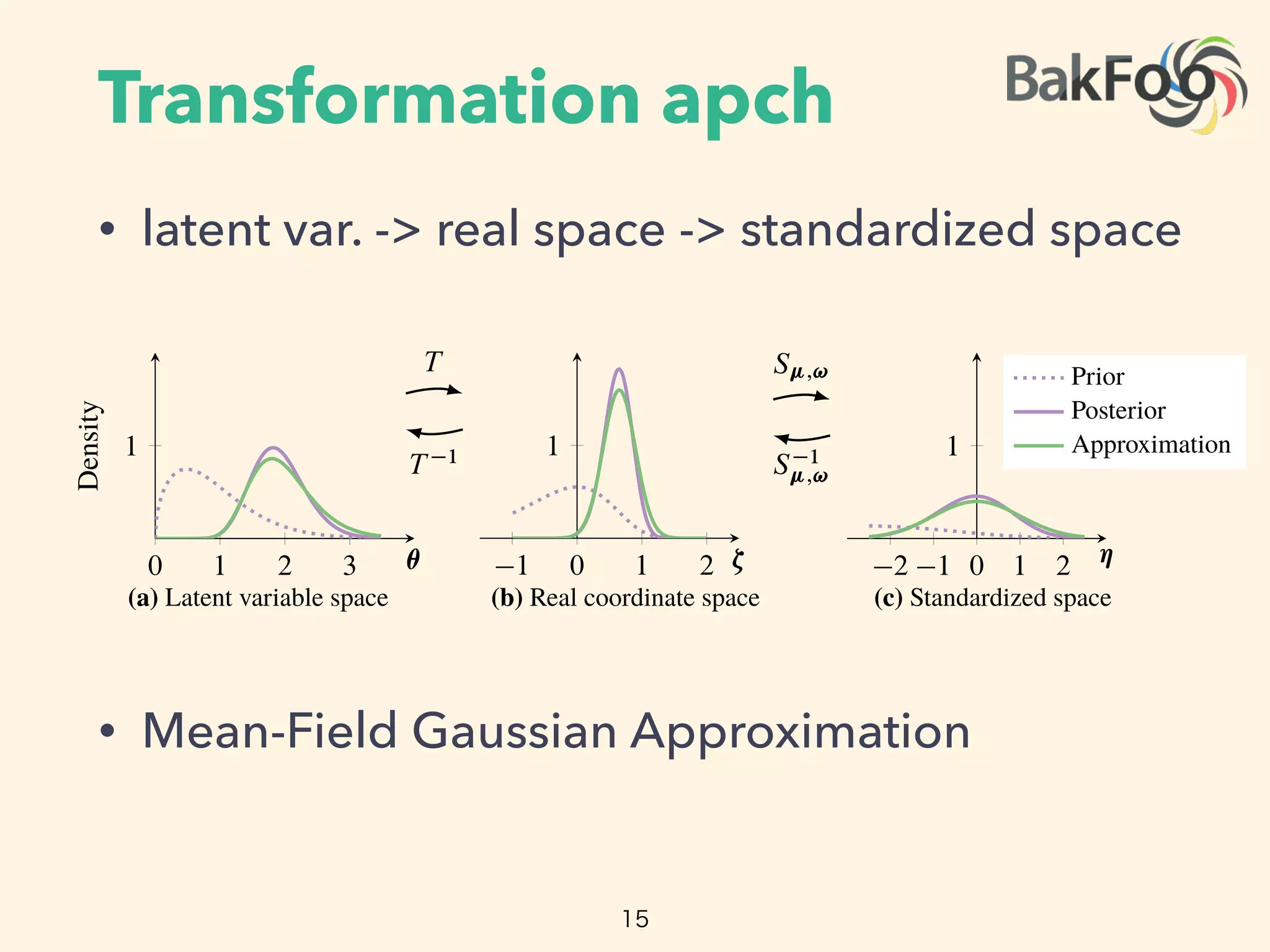
Figure 3: Transformations for . The purple line is the posterior. The gree
mation. (a) The latent variable space is RC
. (a!b) T transforms the latent var
The variational approximation is a Gaussian. (b!c) S ;! absorbs the parame
(c) We maximize the in the standardized space, with a fixed standard Gau
The vector D . 1; ; K; 1; ; K/ contains the mean and standard dev
sian factor. This defines our variational approximation in the real coordinate sp
The transformation T maps the support of the latent variables to the real coordin
T 1
maps back to the support of the latent variables. This implicitly defines th
imation in the original latent variable space as q.T .✓/ I /
ˇ
ˇ det JT .✓/
ˇ
ˇ: The tra
that the support of this approximation is always bounded by that of the true pos
latent variable space (Figure 3a). Thus we can freely optimize the in the r
(Figure 3b) without worrying about the support matching constraint.
The in the real coordinate space is
0 1 2 3
1
✓
Density
(a) Latent variable space
T
T 1
1 0 1 2
1
⇣
(b) Real coordinate space
S ;!
S 1
;!
Figure 3: Transformations for . The purple line is the posterio](https://image.slidesharecdn.com/nips-yomi2016-01-20-160120081335/75/Automatic-Variational-Inference-in-Stan-NIPS2015_yomi2016-01-20-17-2048.jpg)
![MF Gaussian v approx
• ELBO of real space (Appendix A)
• MF Gaussian v approx: for efficiency
• original latent var. space is not Gaussian
18
The vector D . 1; ; K; 1; ; K/ contains the mean and standard deviation of each Gaus-
sian factor. This defines our variational approximation in the real coordinate space. (Figure 3b.)
The transformation T maps the support of the latent variables to the real coordinate space; its inverse
T 1
maps back to the support of the latent variables. This implicitly defines the variational approx-
imation in the original latent variable space as q.T .✓/ I /
ˇ
ˇ det JT .✓/
ˇ
ˇ: The transformation ensures
that the support of this approximation is always bounded by that of the true posterior in the original
latent variable space (Figure 3a). Thus we can freely optimize the in the real coordinate space
(Figure 3b) without worrying about the support matching constraint.
The in the real coordinate space is
L. ; / D Eq.⇣/
log p X; T 1
.⇣/ C log
ˇ
ˇ det JT 1 .⇣/
ˇ
ˇ C
K
2
.1 C log.2⇡// C
KX
kD1
log k;
where we plug in the analytic form of the Gaussian entropy. (The derivation is in Appendix A.)
We choose a diagonal Gaussian for e ciency. This choice may call to mind the Laplace approxima-
tion technique, where a second-order Taylor expansion around the maximum-a-posteriori estimate
gives a Gaussian approximation to the posterior. However, using a Gaussian variational approxima-
tion is not equivalent to the Laplace approximation [18]. The Laplace approximation relies on max-
imizing the probability density; it fails with densities that have discontinuities on its boundary. The
Gaussian approximation considers probability mass; it does not su er this degeneracy. Furthermore,
our approach is distinct in another way: because of the transformation, the posterior approximation
in the original latent variable space (Figure 3a) is non-Gaussian.
2.5 Automatic Di erentiation for Stochastic Optimization
We now maximize the in real coordinate space,
⇤
; ⇤
D arg max
;
L. ; / such that 0: (3)
We use gradient ascent to reach a local maximum of the . Unfortunately, we cannot apply auto-
matic di erentiation to the in this form. This is because the expectation defines an intractable
integral that depends on and ; we cannot directly represent it as a computer program. More-
over, the standard deviations in must remain positive. Thus, we employ one final transformation:
Gaussian Entropy
0 1 2 3
1
✓
Density
(a) Latent variable space
T
T 1
1 0 1 2
1
⇣
(b) Real coordinate space
S ;!
S 1
;!
2
(c) St
Figure 3: Transformations for . The purple line is the posterior. The
mation. (a) The latent variable space is RC
. (a!b) T transforms the laten
Monte Carlo Integration](https://image.slidesharecdn.com/nips-yomi2016-01-20-160120081335/75/Automatic-Variational-Inference-in-Stan-NIPS2015_yomi2016-01-20-18-2048.jpg)
![Standardization
• maximize ELBO in Real space
• intractable integral that depends on μ and σ
• elliptical standardization
• fixed variational density
19
approximation considers probability mass; it does not su er this degeneracy. Furthermore,
ach is distinct in another way: because of the transformation, the posterior approximation
ginal latent variable space (Figure 3a) is non-Gaussian.
omatic Di erentiation for Stochastic Optimization
maximize the in real coordinate space,
⇤
; ⇤
D arg max
;
L. ; / such that 0: (3)
adient ascent to reach a local maximum of the . Unfortunately, we cannot apply auto-
erentiation to the in this form. This is because the expectation defines an intractable
hat depends on and ; we cannot directly represent it as a computer program. More-
standard deviations in must remain positive. Thus, we employ one final transformation:
standardization5
[19], shown in Figures 3b and 3c.
arameterize the Gaussian distribution with the log of the standard deviation, ! D log. /,
ement-wise. The support of ! is now the real coordinate space and is always positive.
ne the standardization ⌘ D S ;!.⇣/ D diag exp .!/ 1 .⇣ /. The standardization
known as a “co-ordinate transformation” [7], an “invertible transformation” [10], and the “re-
zation trick” [6].
5
2.5 Automatic Di erentiation for Stochastic Optimization
We now maximize the in real coordinate space,
⇤
; ⇤
D arg max
;
L. ; / such that 0: (
We use gradient ascent to reach a local maximum of the . Unfortunately, we cannot apply aut
matic di erentiation to the in this form. This is because the expectation defines an intractab
ntegral that depends on and ; we cannot directly represent it as a computer program. Mor
over, the standard deviations in must remain positive. Thus, we employ one final transformatio
elliptical standardization5
[19], shown in Figures 3b and 3c.
First re-parameterize the Gaussian distribution with the log of the standard deviation, ! D log.
applied element-wise. The support of ! is now the real coordinate space and is always positiv
Then define the standardization ⌘ D S ;!.⇣/ D diag exp .!/ 1 .⇣ /. The standardizati
5Also known as a “co-ordinate transformation” [7], an “invertible transformation” [10], and the “
parameterization trick” [6].
5
2.5 Automatic Differentiation for Stochastic Op
We now seek to maximize the elbo in real coordinate space,
µ⇤
, 2⇤
= arg max
µ, 2
L(µ, 2
) such that 2
We can use gradient ascent to reach a local maximum of the elbo.
apply automatic differentiation to the elbo in this form. This is
defines an intractable integral that depends on µ and 2
; we ca
as a computer program. Moreover, the variance vector 2
must r
employ one final transformation: elliptical standardization6
[19],
3c.
First, re-parameterize the Gaussian distribution with the log o
! = log( ), applied element-wise. The support of ! is now the real
always positive. Then, define the standardization ⌘ = Sµ,!(⇣) = di
standardization encapsulates the variational parameters; in return
density
q(⌘ ; 0, I) = N(⌘ ; 0, I) =
KY
k=1
N(⌘k ; 0, 1)
6Also known as a “co-ordinate transformation” [7], an “invertible trans
utomatic Differentiation for Stochastic Optimization
eek to maximize the elbo in real coordinate space,
µ⇤
, 2⇤
= arg max
µ, 2
L(µ, 2
) such that 2
0. (4)
e gradient ascent to reach a local maximum of the elbo. Unfortunately, we cannot
omatic differentiation to the elbo in this form. This is because the expectation
intractable integral that depends on µ and 2
; we cannot directly represent it
uter program. Moreover, the variance vector 2
must remain positive. Thus, we
e final transformation: elliptical standardization6
[19], shown in Figures 3b and
re-parameterize the Gaussian distribution with the log of the standard deviation,
), applied element-wise. The support of ! is now the real coordinate space and is
sitive. Then, define the standardization ⌘ = Sµ,!(⇣) = diag(exp(! 1
))(⇣ µ). The
ation encapsulates the variational parameters; in return it gives a fixed variational
q(⌘ ; 0, I) = N(⌘ ; 0, I) =
KY
k=1
N(⌘k ; 0, 1).
own as a “co-ordinate transformation” [7], an “invertible transformation” [10], and the “re-
ation trick” [6]. 0 1 2 3
1
✓
Density
(a) Latent variable space
T
T 1
1 0 1 2
1
⇣
(b) Real coordinate space
S ;!
S 1
;!
2 1 0 1 2
1
⌘
Prior
Posterior
Approximation
(c) Standardized space](https://image.slidesharecdn.com/nips-yomi2016-01-20-160120081335/75/Automatic-Variational-Inference-in-Stan-NIPS2015_yomi2016-01-20-19-2048.jpg)
![Gradient of ELBO
• maximaize ELBO
• expectation is in terms of standard Gaussian
• gradient of ELBO(Appendix B)
20
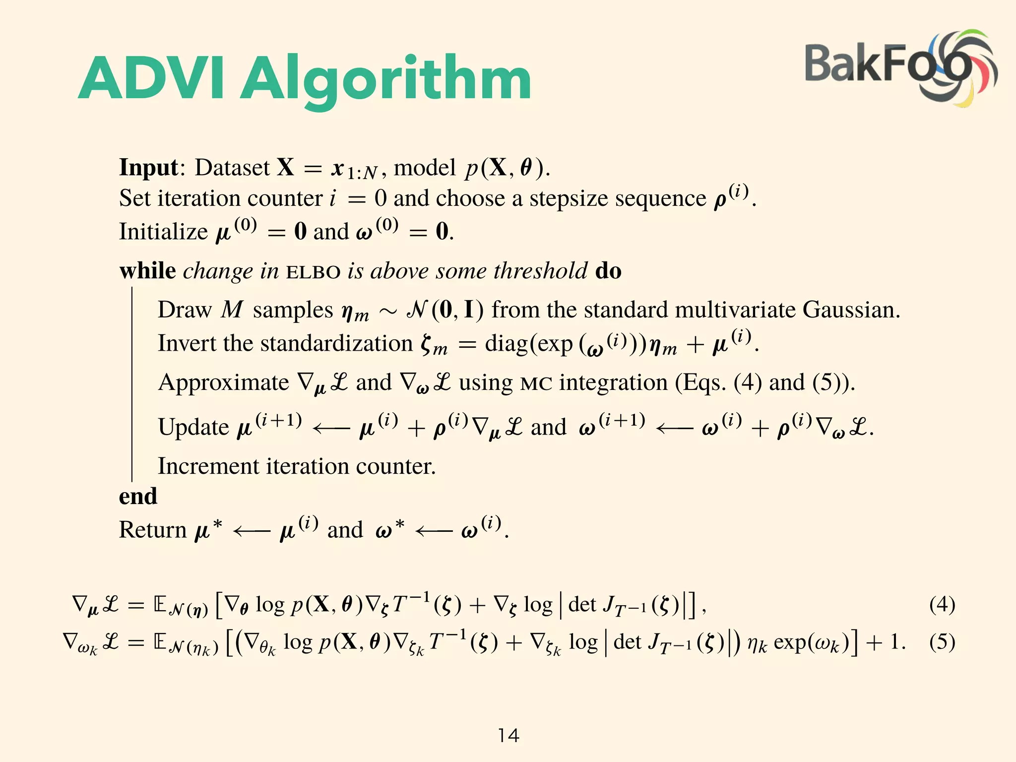
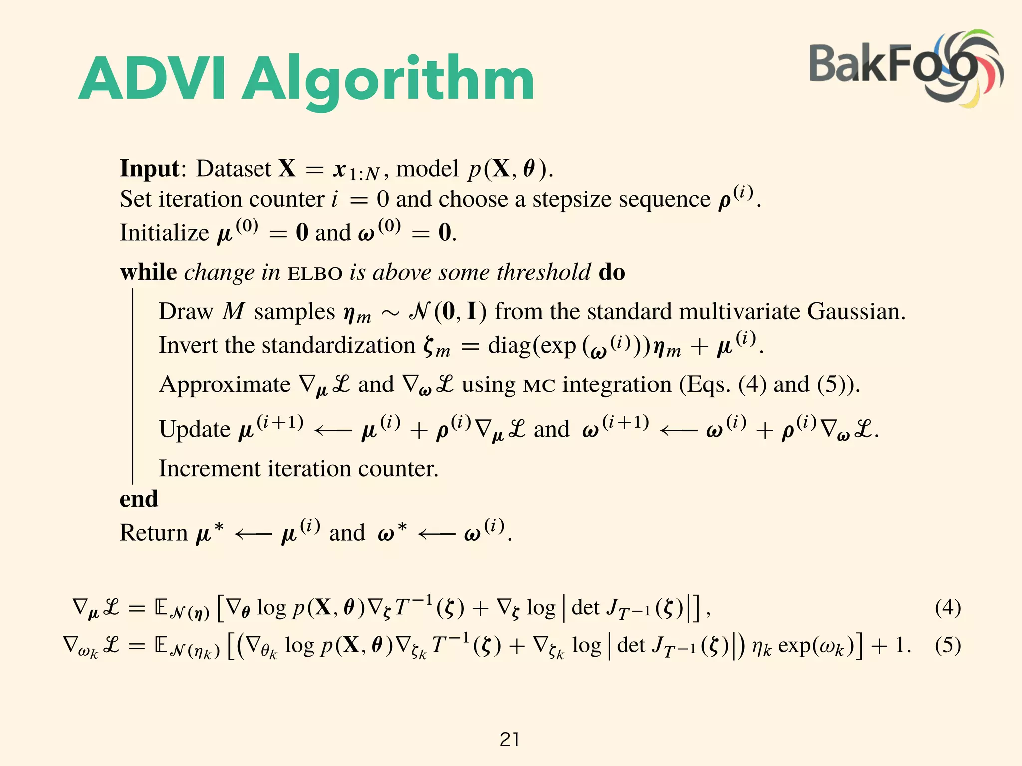
Update µ(i+1)
µ(i)
+ ⇢(i)
rµL and !(i+1)
!(i)
+ ⇢(i)
r!L.
Increment iteration counter.
end
Return µ⇤
µ(i)
and !⇤
!(i)
.
The standardization transforms the variational problem from Equation 4 into
µ⇤
, !⇤
= arg max
µ,!
L(µ, !)
= arg max
µ,!
EN (⌘ ; 0,I)
log p(X, T 1
(S 1
µ,!(⌘))) + log det JT 1 (S 1
µ,!(⌘)) +
KX
k=1
!k,
where we drop independent term from the calculation. The expectation is now in terms of
the standard Gaussian, and both parameters µ and ! are unconstrained. (Figure 3c.) We
push the gradient inside the expectations and apply the chain rule to get
rµL = EN (⌘)
⇥
r✓ log p(X, ✓)r⇣T 1
(⇣) + r⇣ log det JT 1 (⇣)
⇤
, (5)
r!k
L = EN (⌘k)
⇥
r✓k
log p(X, ✓)r⇣k
T 1
(⇣) + r⇣k
log det JT 1 (⇣) ⌘k exp(!k)
⇤
+ 1. (6)
(Derivations in Appendix B.)
We can now compute the gradients inside the expectation with automatic differentiation.
This leaves only the expectation. mc integration provides a simple approximation: draw
M samples from the standard Gaussian and evaluate the empirical mean of the gradients
within the expectation [20]. This gives unbiased noisy estimates of gradients of the elbo.
2.6 Scalable Automatic Variational Inference
Equipped with unbiased noisy gradients of the elbo, advi implements stochastic gradient
Update µ(i+1)
µ(i)
+ ⇢(i)
rµL and !(i+1)
!(i)
+ ⇢(i)
r!L.
Increment iteration counter.
end
Return µ⇤
µ(i)
and !⇤
!(i)
.
The standardization transforms the variational problem from Equation 4 into
µ⇤
, !⇤
= arg max
µ,!
L(µ, !)
= arg max
µ,!
EN (⌘ ; 0,I)
log p(X, T 1
(S 1
µ,!(⌘))) + log det JT 1 (S 1
µ,!(⌘)) +
KX
k=1
!k,
where we drop independent term from the calculation. The expectation is now in terms of
the standard Gaussian, and both parameters µ and ! are unconstrained. (Figure 3c.) We
push the gradient inside the expectations and apply the chain rule to get
rµL = EN (⌘)
⇥
r✓ log p(X, ✓)r⇣T 1
(⇣) + r⇣ log det JT 1 (⇣)
⇤
, (5)
r!k
L = EN (⌘k)
⇥
r✓k
log p(X, ✓)r⇣k
T 1
(⇣) + r⇣k
log det JT 1 (⇣) ⌘k exp(!k)
⇤
+ 1. (6)
(Derivations in Appendix B.)
We can now compute the gradients inside the expectation with automatic differentiation.
This leaves only the expectation. mc integration provides a simple approximation: draw
M samples from the standard Gaussian and evaluate the empirical mean of the gradients
within the expectation [20]. This gives unbiased noisy estimates of gradients of the elbo.](https://image.slidesharecdn.com/nips-yomi2016-01-20-160120081335/75/Automatic-Variational-Inference-in-Stan-NIPS2015_yomi2016-01-20-20-2048.jpg)
![Lin. Regression /w ARD
24
10 1
100
101
9
7
5
3
Seconds
AverageLogPredictive
ADVI (M=1)
ADVI (M=10)
NUTS
HMC
(a) Linear Regression with
Figure 4: Hierarchical generalized linear model
tive likelihood as a function of wall time.
3 Empirical Study
We now study across a variety of models.
chain Monte Carlo ( ) sampling algorithms
U-turn sampler ( )6
[5]. We assess con
on a common scale, we report predictive l
approximate the posterior predictive likelihood u
data {
int < lower=0> N; // number of data items
int < lower=0> D; // dimension of input f e a t u r e s
matrix [N,D] x ; // input matrix
vector [N] y ; // output vector
// hyperparameters f o r Gamma p r i o r s
real < lower=0> a0 ;
real < lower=0> b0 ;
real < lower=0> c0 ;
real < lower=0> d0 ;
}
parameters {
vector [D] w; // weights ( c o e f f i c i e n t s ) vector
real < lower=0> sigma2 ; // variance
vector < lower =0>[D] alpha ; // hyper - parameters on weights
}
transformed parameters {
r e a l sigma ; // standard deviation
vector [D] one_over_sqrt_alpha ; // numerical s t a b i l i t y
sigma < - sqrt ( sigma2 ) ;
f o r ( i in 1:D) {
one_over_sqrt_alpha [ i ] < - 1 / sqrt ( alpha [ i ] ) ;
}
}
model {
// alpha : hyper - p r i o r on weights
alpha ~ gamma( c0 , d0 ) ;
// sigma2 : p r i o r on variance
sigma2 ~ inv_gamma( a0 , b0 ) ;
// w: p r i o r on weights
w ~ normal (0 , sigma * one_over_sqrt_alpha ) ;
// y : l i k e l i h o o d
y ~ normal (x * w, sigma ) ;
}
Figure 6: Stan code for Linear Regression with Automatic Relevance Determination.](https://image.slidesharecdn.com/nips-yomi2016-01-20-160120081335/75/Automatic-Variational-Inference-in-Stan-NIPS2015_yomi2016-01-20-24-2048.jpg)
![Hierarchical Logistic Reg
25
10 1
100
101
9
7
5
3
Seconds
AverageLogPredictive
ADVI (M=1)
ADVI (M=10)
NUTS
HMC
(a) Linear Regression with
10 1
100
101
102
1:5
1:3
1:1
0:9
0:7
Seconds
AverageLogPredictive
ADVI (M=1)
ADVI (M=10)
NUTS
HMC
(b) Hierarchical Logistic Regression
Figure 4: Hierarchical generalized linear models. Comparison of to : held-out predic-
tive likelihood as a function of wall time.
3 Empirical Study
We now study across a variety of models. We compare its speed and accuracy to two Markov
chain Monte Carlo ( ) sampling algorithms: Hamiltonian Monte Carlo ( ) [22] and the no-
U-turn sampler ( )6
[5]. We assess convergence by tracking the . To place and
on a common scale, we report predictive likelihood on held-out data as a function of time. We
approximate the posterior predictive likelihood using a estimate. For , we plug in posterior
data {
int < lower=0> N;
int < lower=0> n_age ;
int < lower=0> n_age_edu ;
int < lower=0> n_edu ;
int < lower=0> n_region_full ;
int < lower=0> n_state ;
int < lower =0,upper=n_age> age [N ] ;
int < lower =0,upper=n_age_edu> age_edu [N ] ;
vector < lower =0,upper=1>[N] black ;
int < lower =0,upper=n_edu> edu [N ] ;
vector < lower =0,upper=1>[N] female ;
int < lower =0,upper=n_region_full > r e g i o n _ f u l l [N ] ;
int < lower =0,upper=n_state > s t a t e [N ] ;
vector [N] v_prev_full ;
int < lower =0,upper=1> y [N ] ;
}
parameters {
vector [ n_age ] a ;
vector [ n_edu ] b ;
vector [ n_age_edu ] c ;
vector [ n_state ] d ;
vector [ n_region_full ] e ;
vector [ 5 ] beta ;
real < lower =0,upper=100> sigma_a ;
real < lower =0,upper=100> sigma_b ;
real < lower =0,upper=100> sigma_c ;
real < lower =0,upper=100> sigma_d ;
real < lower =0,upper=100> sigma_e ;
}
transformed parameters {
vector [N] y_hat ;
f o r ( i in 1:N)
y_hat [ i ] < - beta [ 1 ]
+ beta [ 2 ] * black [ i ]
+ beta [ 3 ] * female [ i ]
+ beta [ 5 ] * female [ i ] * black [ i ]
+ beta [ 4 ] * v_prev_full [ i ]
+ a [ age [ i ] ]
+ b [ edu [ i ] ]
+ c [ age_edu [ i ] ]
+ d [ s t a t e [ i ] ]
+ e [ r e g i o n _ f u l l [ i ] ] ;
}
model {
a ~ normal (0 , sigma_a ) ;
b ~ normal (0 , sigma_b ) ;
c ~ normal (0 , sigma_c ) ;
d ~ normal (0 , sigma_d ) ;
e ~ normal (0 , sigma_e ) ;
beta ~ normal (0 , 100) ;
y ~ b e r n o u l l i _ l o g i t ( y_hat ) ;
}](https://image.slidesharecdn.com/nips-yomi2016-01-20-160120081335/75/Automatic-Variational-Inference-in-Stan-NIPS2015_yomi2016-01-20-25-2048.jpg)
![Gamma Poisson Non-Neg
26
101
102
103
104
11
9
7
5
Seconds
AverageLogPredictive
ADVI
NUTS
(a) Gamma Poisson Predictive Likelihood
AverageLogPredictive
(b)
(c) Gamma Poisson Factors
Figure 5: Non-negative matrix factorization of the F
: held-out predictive likelihood as a function of w
Dirichlet Exponential. This is a nonconjugate Diric
Poisson likelihood. (Details in Appendix I.)
data {
int < lower=0> U;
int < lower=0> I ;
int < lower=0> K;
int < lower=0> y [U, I ] ;
real < lower=0> a ;
real < lower=0> b ;
real < lower=0> c ;
real < lower=0> d ;
}
parameters {
positive_ordered [K] theta [U ] ; // user p r e f e r e n c e
vector < lower =0>[K] beta [ I ] ; // item a t t r i b u t e s
}
model {
f o r (u in 1:U)
theta [ u ] ~ gamma( a , b) ; // componentwise gamma
f o r ( i in 1: I )
beta [ i ] ~ gamma( c , d) ; // componentwise gamma
f o r (u in 1:U) {
f o r ( i in 1: I ) {
increment_log_prob (
poisson_log ( y [ u , i ] , theta [ u ] ‘ * beta [ i ] ) ) ;
}
}
}
igure 8: Stan code for Gamma Poisson non-negative matrix factorization model.](https://image.slidesharecdn.com/nips-yomi2016-01-20-160120081335/75/Automatic-Variational-Inference-in-Stan-NIPS2015_yomi2016-01-20-26-2048.jpg)
![Dirichlet Exponential NonNeg
27
101
102
103
104
11
9
7
5
Seconds
AverageLogPredictive
ADVI
NUTS
(a) Gamma Poisson Predictive Likelihood
101
102
103
104
600
400
200
0
Seconds
AverageLogPredictive
ADVI
NUTS
(b) Dirichlet Exponential Predictive Likelihood
(c) Gamma Poisson Factors (d) Dirichlet Exponential Factors
Figure 5: Non-negative matrix factorization of the Frey Faces dataset. Comparison of to
: held-out predictive likelihood as a function of wall time.
Dirichlet Exponential. This is a nonconjugate Dirichlet Exponential factorization model with a
Poisson likelihood. (Details in Appendix I.)
Figure 8: Stan code for Gamma Poisson non-negative matrix factorization model.
data {
int < lower=0> U;
int < lower=0> I ;
int < lower=0> K;
int < lower=0> y [U, I ] ;
real < lower=0> lambda0 ;
real < lower=0> alpha0 ;
}
transformed data {
vector < lower =0>[K] alpha0_vec ;
f o r (k in 1:K) {
alpha0_vec [ k ] < - alpha0 ;
}
}
parameters {
simplex [K] theta [U ] ; // user p r e f e r e n c e
vector < lower =0>[K] beta [ I ] ; // item a t t r i b u t e s
}
model {
f o r (u in 1:U)
theta [ u ] ~ d i r i c h l e t ( alpha0_vec ) ; // componentwise d i r i c h l e t
f o r ( i in 1: I )
beta [ i ] ~ exponential ( lambda0 ) ; // componentwise gamma
f o r (u in 1:U) {
f o r ( i in 1: I ) {
increment_log_prob (
poisson_log ( y [ u , i ] , theta [ u ] ‘ * beta [ i ] ) ) ;
}
}
}
gure 9: Stan code for Dirichlet Exponential non-negative matrix factorization model.](https://image.slidesharecdn.com/nips-yomi2016-01-20-160120081335/75/Automatic-Variational-Inference-in-Stan-NIPS2015_yomi2016-01-20-27-2048.jpg)
![GMM
28
data {
int < lower=0> N; // number of data points in e n t i r e dataset
int < lower=0> K; // number of mixture components
int < lower=0> D; // dimension
vector [D] y [N ] ; // observations
real < lower=0> alpha0 ; // d i r i c h l e t p r i o r
real < lower=0> mu_sigma0 ; // means p r i o r
real < lower=0> sigma_sigma0 ; // variances p r i o r
}
transformed data {
vector < lower =0>[K] alpha0_vec ;
f o r (k in 1:K) {
alpha0_vec [ k ] < - alpha0 ;
}
}
parameters {
simplex [K] theta ; // mixing proportions
vector [D] mu[K] ; // l o c a t i o n s of mixture components
vector < lower =0>[D] sigma [K] ; // standard d e v i a t i o n s of mixture components
}
model {
// p r i o r s
theta ~ d i r i c h l e t ( alpha0_vec ) ;
f o r (k in 1:K) {
mu[ k ] ~ normal ( 0 . 0 , mu_sigma0) ;
sigma [ k ] ~ lognormal ( 0 . 0 , sigma_sigma0 ) ;
}
// l i k e l i h o o d
f o r (n in 1:N) {
r e a l ps [K] ;
f o r (k in 1:K) {
ps [ k ] < - log ( theta [ k ] ) + normal_log (y [ n ] , mu[ k ] , sigma [ k ] ) ;
}
increment_log_prob ( log_sum_exp ( ps ) ) ;
}
}
Figure 10: advi Stan code for the gmm example.
102
103
900
600
300
0
Seconds
AverageLogPredictive
ADVI
NUTS [5]
(a) Subset of 1000 images
Figure 1: Held-out predictive accuracy results | Gauss
image histogram dataset. (a) outperforms the no-
method in Stan [5]. (b) scales to large datasets by
dataset at each iteration [3]. We present more details in
Figure 1 illustrates the advantages of our method. Cons
for analyzing natural images; this is 40 lines in Stan
inference on 1000 images. The y-axis is held-out lik
axis is time on a log scale. is orders of magnitu
algorithm (and Stan’s default inference technique) [5]
models and hierarchical generalized linear models in S
Figure 1b illustrates Bayesian inference on 250 000 imag](https://image.slidesharecdn.com/nips-yomi2016-01-20-160120081335/75/Automatic-Variational-Inference-in-Stan-NIPS2015_yomi2016-01-20-28-2048.jpg)
![GMM /w Stoch.Subsamp
29
data {
real < lower=0> N; // number of data points in e n t i r e dataset
int < lower=0> S_in_minibatch ;
int < lower=0> K; // number of mixture components
int < lower=0> D; // dimension
vector [D] y [ S_in_minibatch ] ; // observations
real < lower=0> alpha0 ; // d i r i c h l e t p r i o r
real < lower=0> mu_sigma0 ; // means p r i o r
real < lower=0> sigma_sigma0 ; // variances p r i o r
}
transformed data {
r e a l SVI_factor ;
vector < lower =0>[K] alpha0_vec ;
f o r (k in 1:K) {
alpha0_vec [ k ] < - alpha0 ;
}
SVI_factor < - N / S_in_minibatch ;
}
parameters {
simplex [K] theta ; // mixing proportions
vector [D] mu[K] ; // l o c a t i o n s of mixture components
vector < lower =0>[D] sigma [K] ; // standard d e v i a t i o n s of mixture components
}
model {
// p r i o r s
theta ~ d i r i c h l e t ( alpha0_vec ) ;
f o r (k in 1:K) {
mu[ k ] ~ normal ( 0 . 0 , mu_sigma0) ;
sigma [ k ] ~ lognormal ( 0 . 0 , sigma_sigma0 ) ;
}
// l i k e l i h o o d
f o r (n in 1: S_in_minibatch ) {
r e a l ps [K] ;
f o r (k in 1:K) {
ps [ k ] < - log ( theta [ k ] ) + normal_log (y [ n ] , mu[ k ] , sigma [ k ] ) ;
}
increment_log_prob ( log_sum_exp ( ps ) ) ;
}
increment_log_prob ( log ( SVI_factor ) ) ;
}
Figure 11: advi Stan code for the gmm example, with stochastic subsampling of the
102
103
900
600
300
0
Seconds
AverageLogPredictive
ADVI
NUTS [5]
(a) Subset of 1000 images
102
103
104
800
400
0
400
Seconds
AverageLogPredictive
B=50
B=100
B=500
B=1000
(b) Full dataset of 250 000 images
Figure 1: Held-out predictive accuracy results | Gaussian mixture model ( ) of the image
image histogram dataset. (a) outperforms the no-U-turn sampler ( ), the default sampling
method in Stan [5]. (b) scales to large datasets by subsampling minibatches of size B from the
dataset at each iteration [3]. We present more details in Section 3.3 and Appendix J.
Figure 1 illustrates the advantages of our method. Consider a nonconjugate Gaussian mixture model
for analyzing natural images; this is 40 lines in Stan (Figure 10). Figure 1a illustrates Bayesian
inference on 1000 images. The y-axis is held-out likelihood, a measure of model fitness; the x-
axis is time on a log scale. is orders of magnitude faster than , a state-of-the-art
algorithm (and Stan’s default inference technique) [5]. We also study nonconjugate factorization](https://image.slidesharecdn.com/nips-yomi2016-01-20-160120081335/75/Automatic-Variational-Inference-in-Stan-NIPS2015_yomi2016-01-20-29-2048.jpg)
![Stochastic Subsampling?
30
data {
int < lower=0> N; // number of data points in e n t i r e dataset
int < lower=0> K; // number of mixture components
int < lower=0> D; // dimension
vector [D] y [N ] ; // observations
real < lower=0> alpha0 ; // d i r i c h l e t p r i o r
real < lower=0> mu_sigma0 ; // means p r i o r
real < lower=0> sigma_sigma0 ; // variances p r i o r
}
transformed data {
vector < lower =0>[K] alpha0_vec ;
f o r (k in 1:K) {
alpha0_vec [ k ] < - alpha0 ;
}
}
parameters {
simplex [K] theta ; // mixing proportions
vector [D] mu[K] ; // l o c a t i o n s of mixture components
vector < lower =0>[D] sigma [K] ; // standard d e v i a t i o n s of mixture components
}
model {
// p r i o r s
theta ~ d i r i c h l e t ( alpha0_vec ) ;
f o r (k in 1:K) {
mu[ k ] ~ normal ( 0 . 0 , mu_sigma0) ;
sigma [ k ] ~ lognormal ( 0 . 0 , sigma_sigma0 ) ;
}
// l i k e l i h o o d
f o r (n in 1:N) {
r e a l ps [K] ;
f o r (k in 1:K) {
ps [ k ] < - log ( theta [ k ] ) + normal_log (y [ n ] , mu[ k ] , sigma [ k ] ) ;
}
increment_log_prob ( log_sum_exp ( ps ) ) ;
}
}
Figure 10: advi Stan code for the gmm example.
data {
real < lower=0> N; // number of data points in e n t i r e dataset
int < lower=0> S_in_minibatch ;
int < lower=0> K; // number of mixture components
int < lower=0> D; // dimension
vector [D] y [ S_in_minibatch ] ; // observations
real < lower=0> alpha0 ; // d i r i c h l e t p r i o r
real < lower=0> mu_sigma0 ; // means p r i o r
real < lower=0> sigma_sigma0 ; // variances p r i o r
}
transformed data {
r e a l SVI_factor ;
vector < lower =0>[K] alpha0_vec ;
f o r (k in 1:K) {
alpha0_vec [ k ] < - alpha0 ;
}
SVI_factor < - N / S_in_minibatch ;
}
parameters {
simplex [K] theta ; // mixing proportions
vector [D] mu[K] ; // l o c a t i o n s of mixture components
vector < lower =0>[D] sigma [K] ; // standard d e v i a t i o n s of mixture compon
}
model {
// p r i o r s
theta ~ d i r i c h l e t ( alpha0_vec ) ;
f o r (k in 1:K) {
mu[ k ] ~ normal ( 0 . 0 , mu_sigma0) ;
sigma [ k ] ~ lognormal ( 0 . 0 , sigma_sigma0 ) ;
}
// l i k e l i h o o d
f o r (n in 1: S_in_minibatch ) {
r e a l ps [K] ;
f o r (k in 1:K) {
ps [ k ] < - log ( theta [ k ] ) + normal_log (y [ n ] , mu[ k ] , sigma [ k ] ) ;
}
increment_log_prob ( log_sum_exp ( ps ) ) ;
}
increment_log_prob ( log ( SVI_factor ) ) ;
}
Figure 11: advi Stan code for the gmm example, with stochastic subsam
dataset.](https://image.slidesharecdn.com/nips-yomi2016-01-20-160120081335/75/Automatic-Variational-Inference-in-Stan-NIPS2015_yomi2016-01-20-30-2048.jpg)


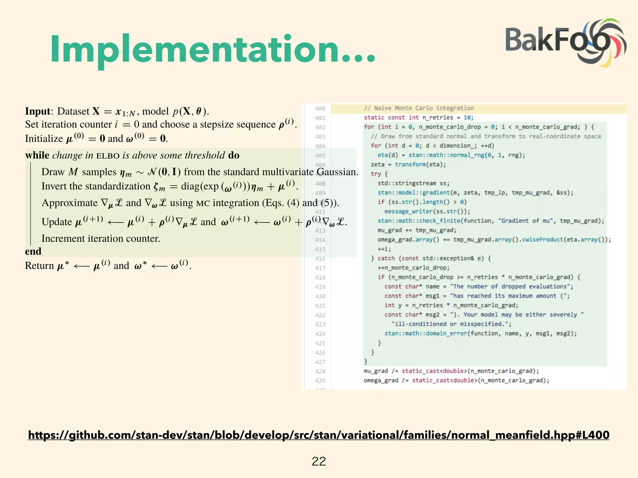
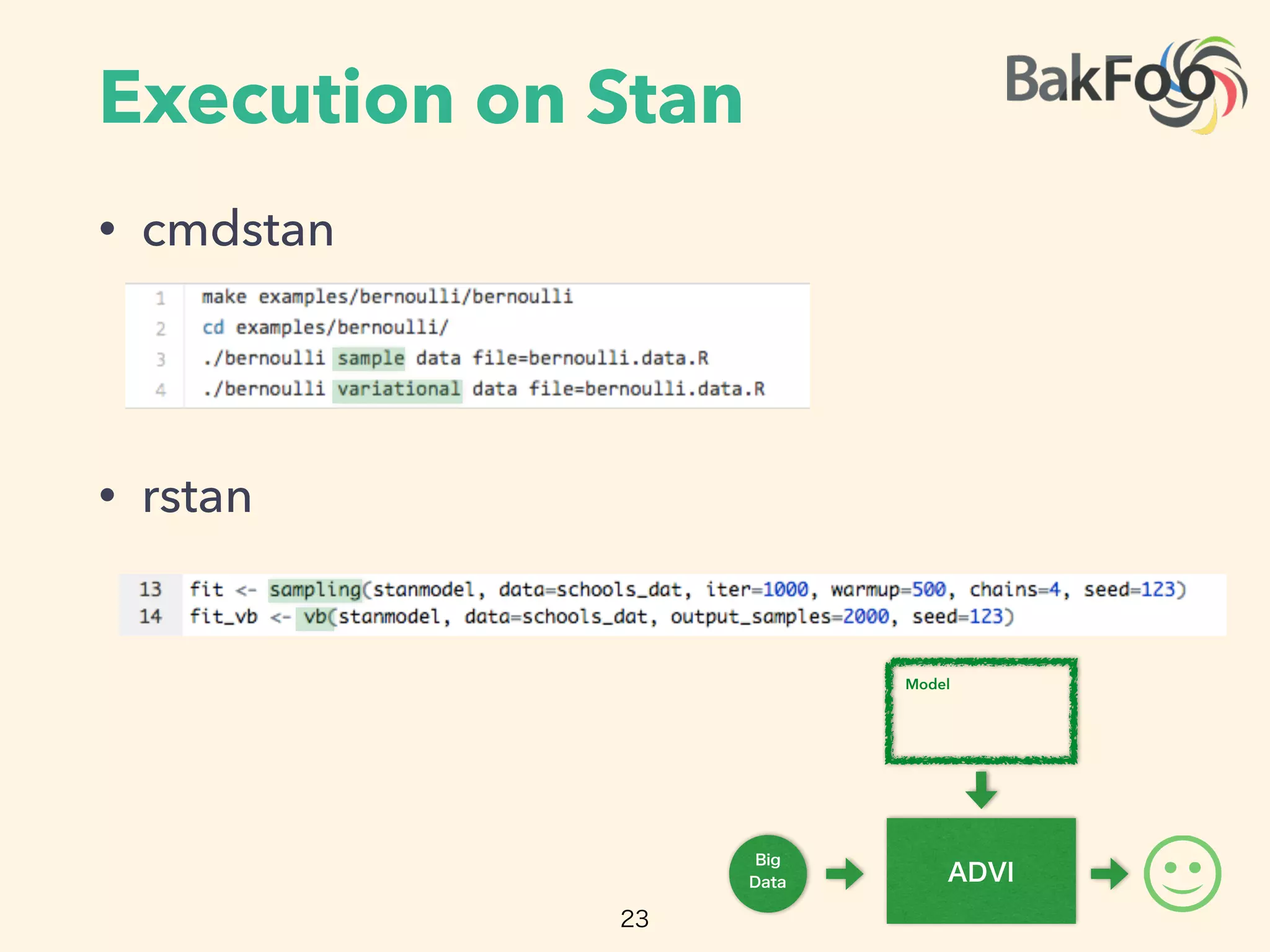
Automatic variational inference (ADVI) can be implemented in Stan to automate variational inference for any probabilistic model specified in Stan. ADVI determines an appropriate variational family and optimizes the variational objective without any input from the user beyond providing the model and data. ADVI handles nonconjugate models by automatically deriving an inference algorithm. It scales to large datasets using subsampling and has been shown to outperform sampling methods while training models with hundreds of thousands of data points.


![[DL輪読会]Generative Models of Visually Grounded Imagination](https://cdn.slidesharecdn.com/ss_thumbnails/20170602-170602005505-thumbnail.jpg?width=640&height=640&fit=bounds)