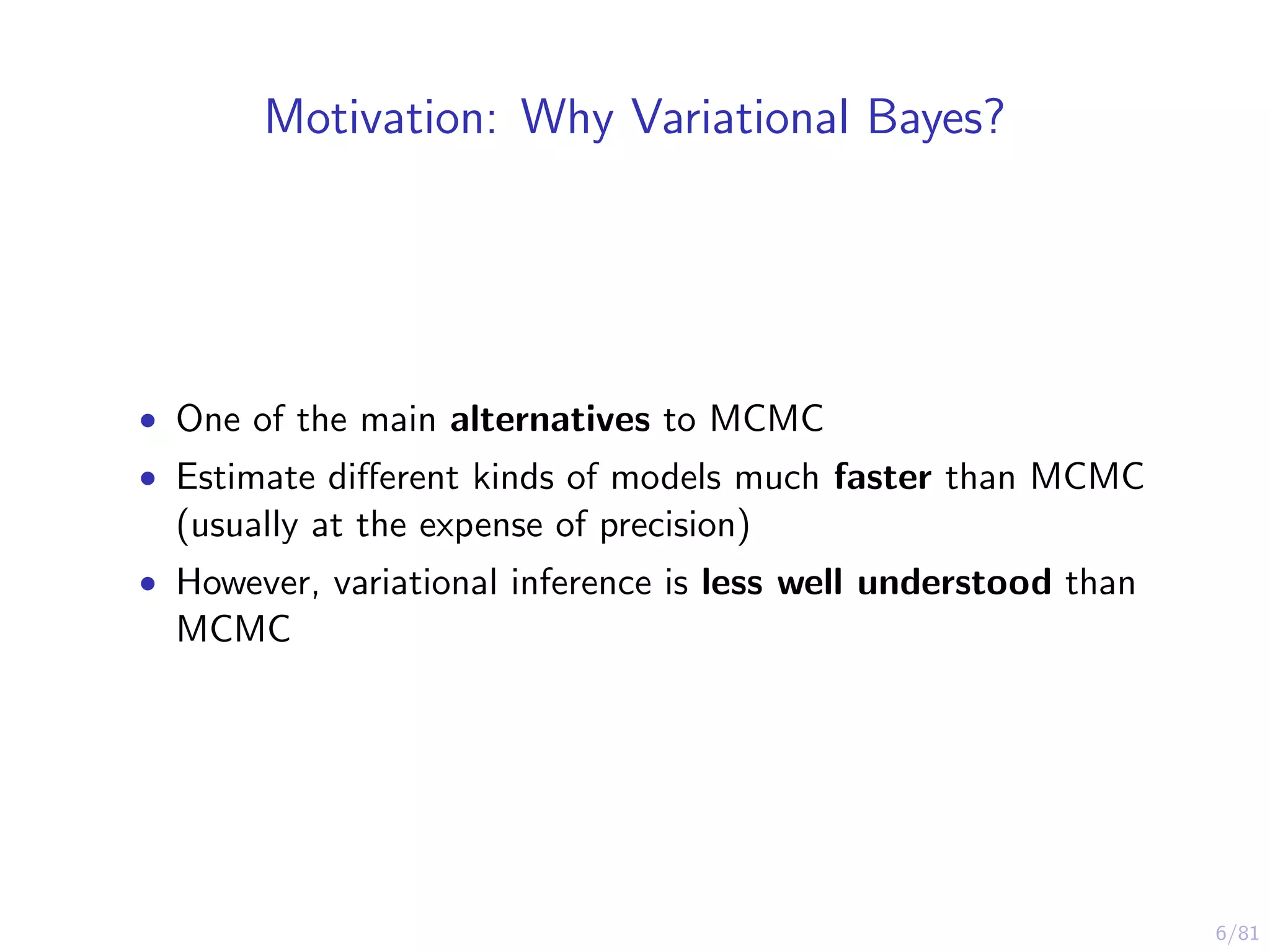
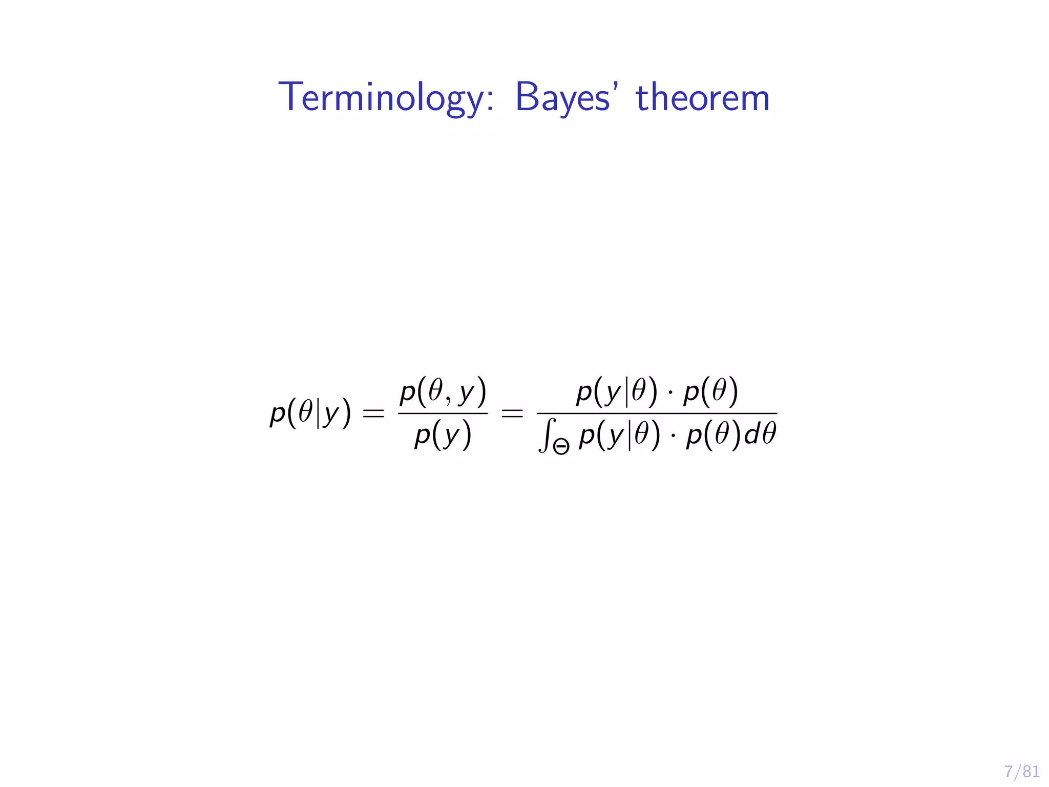
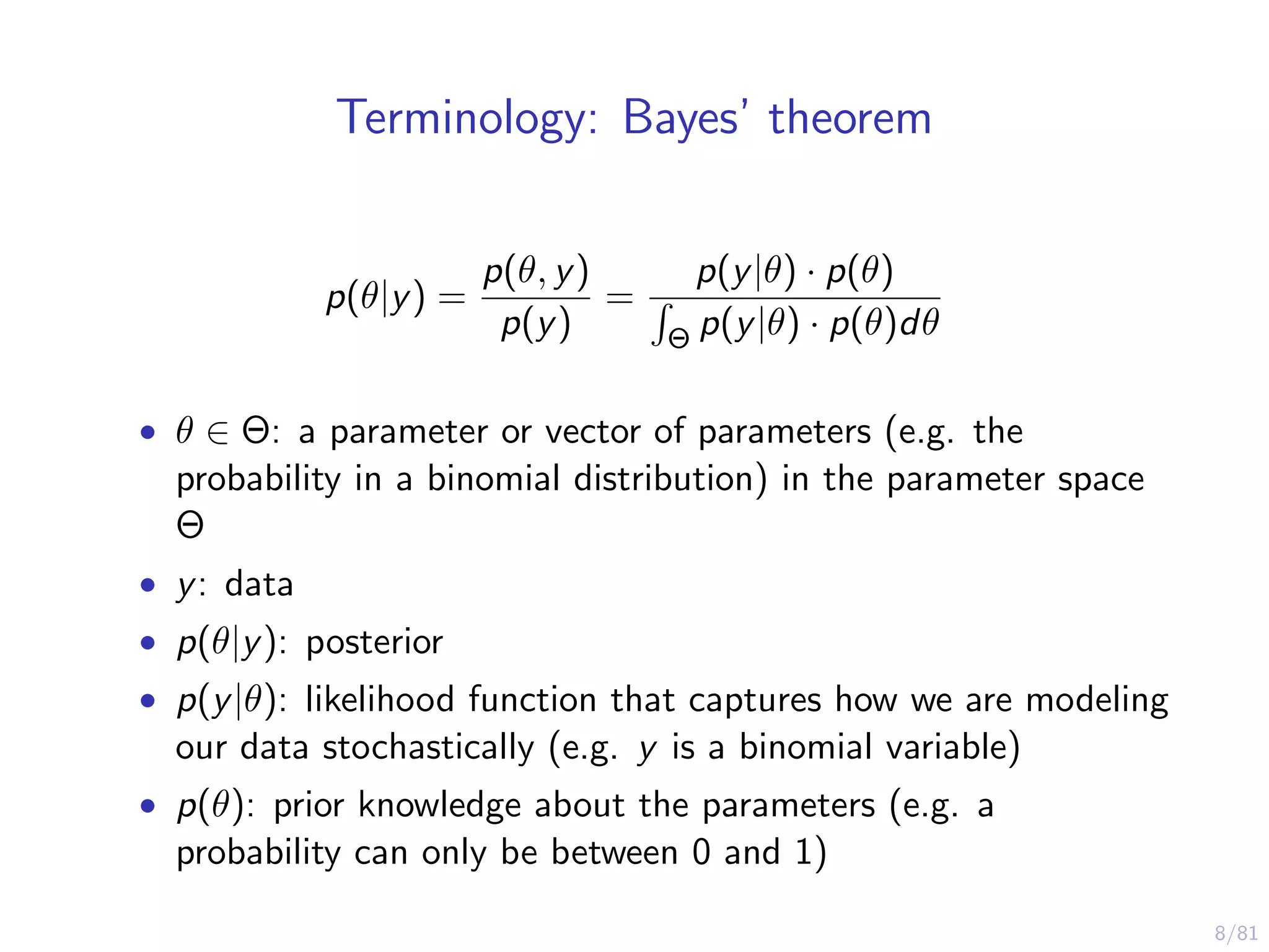
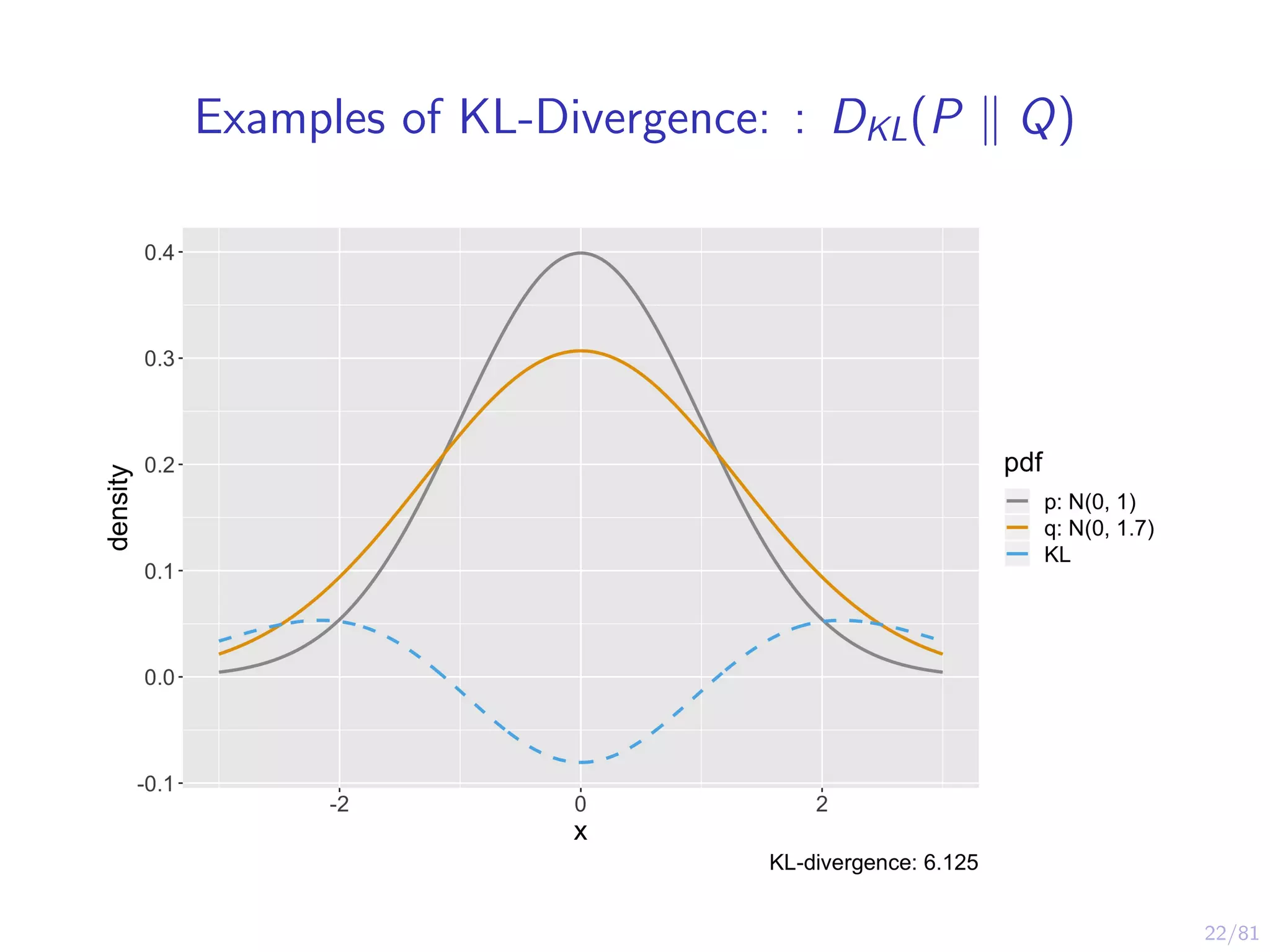
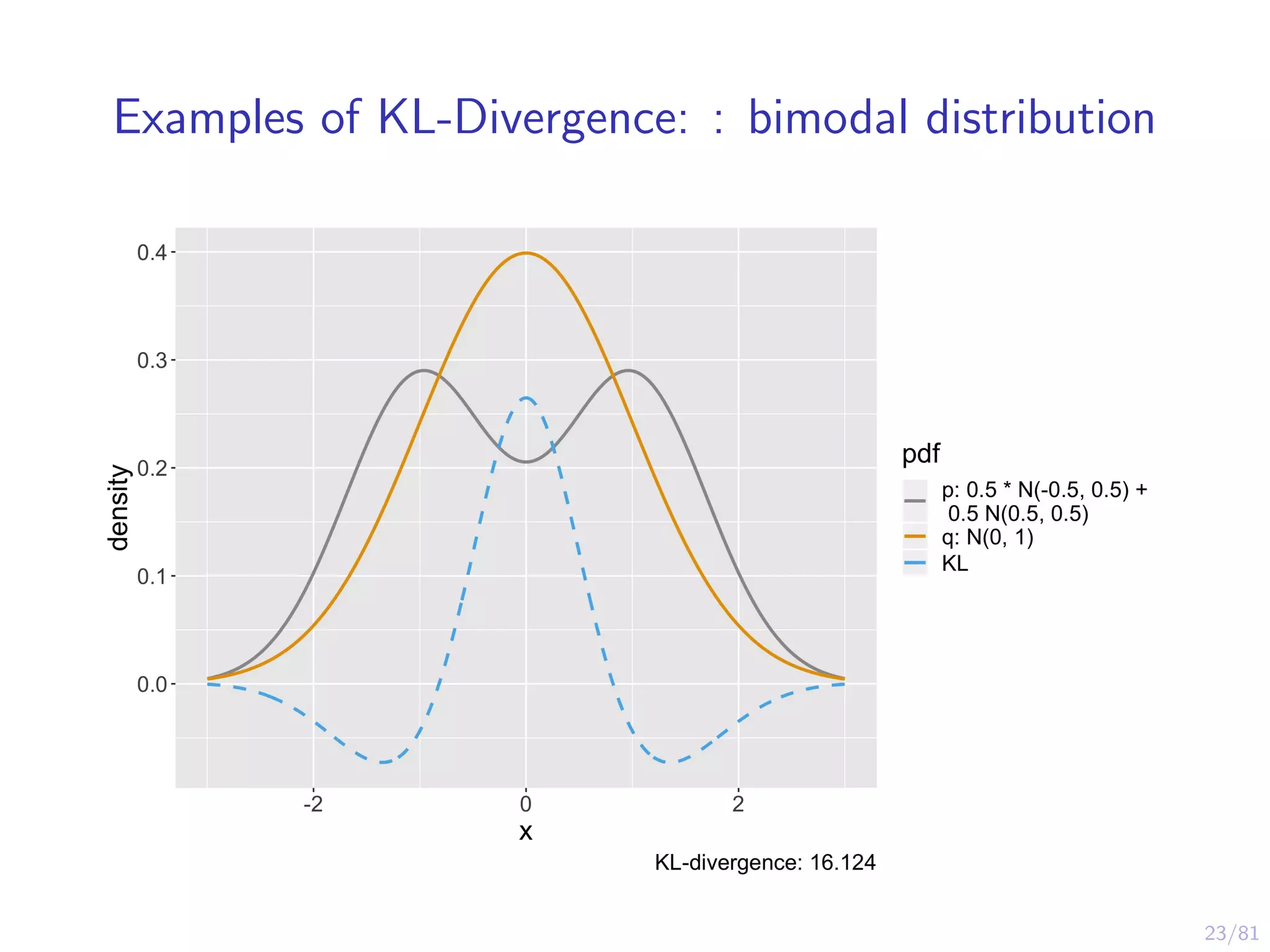
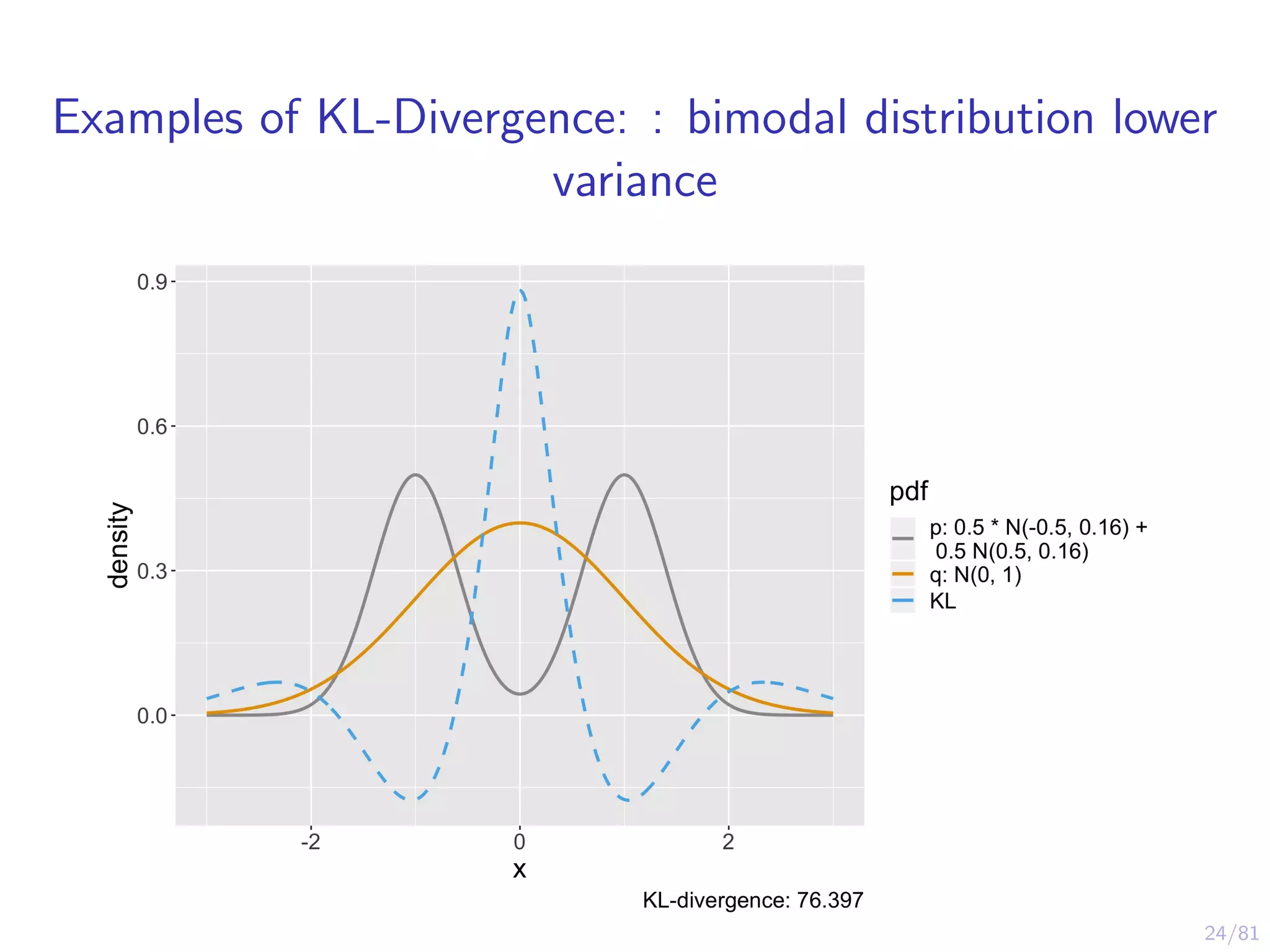
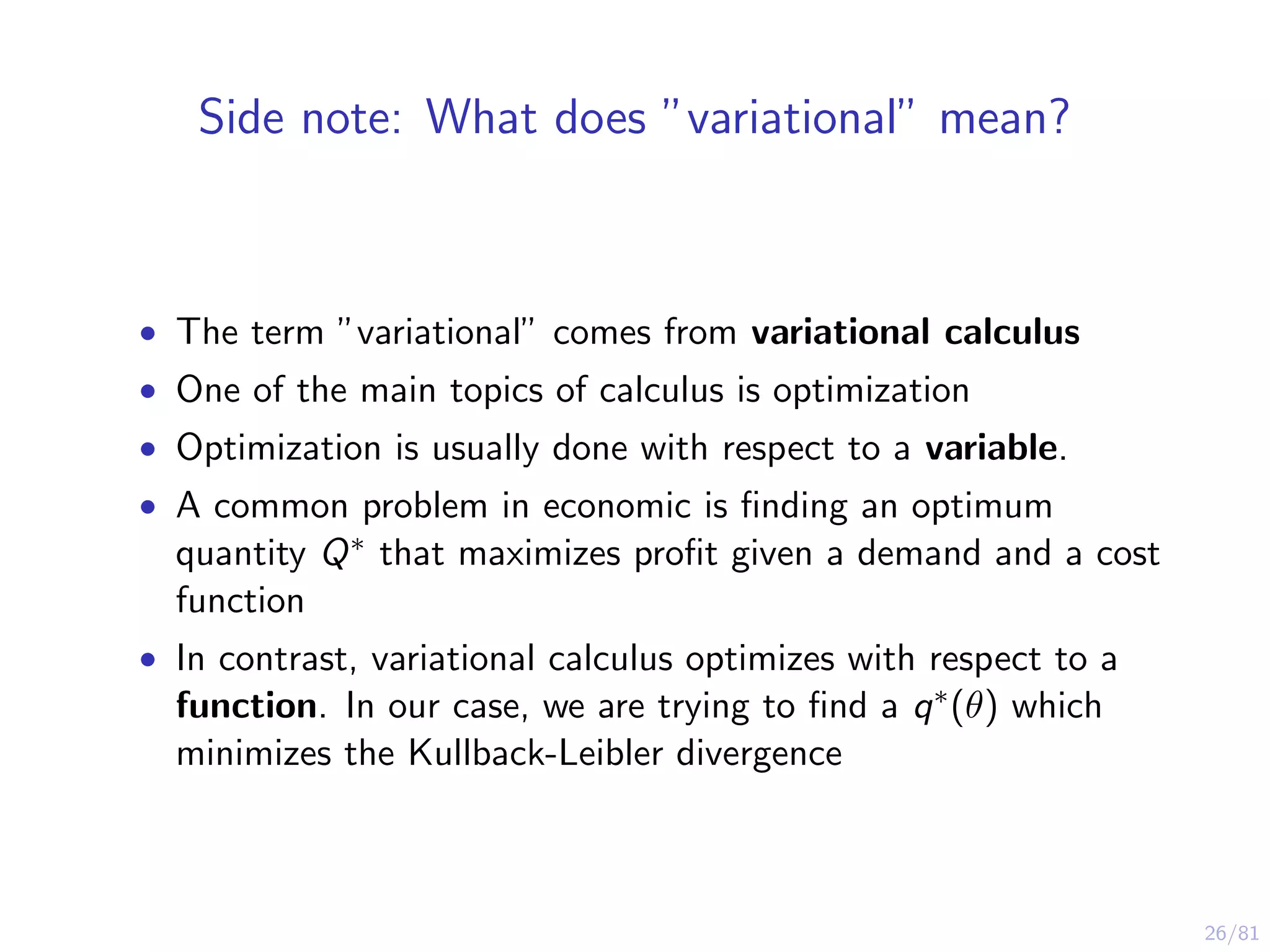
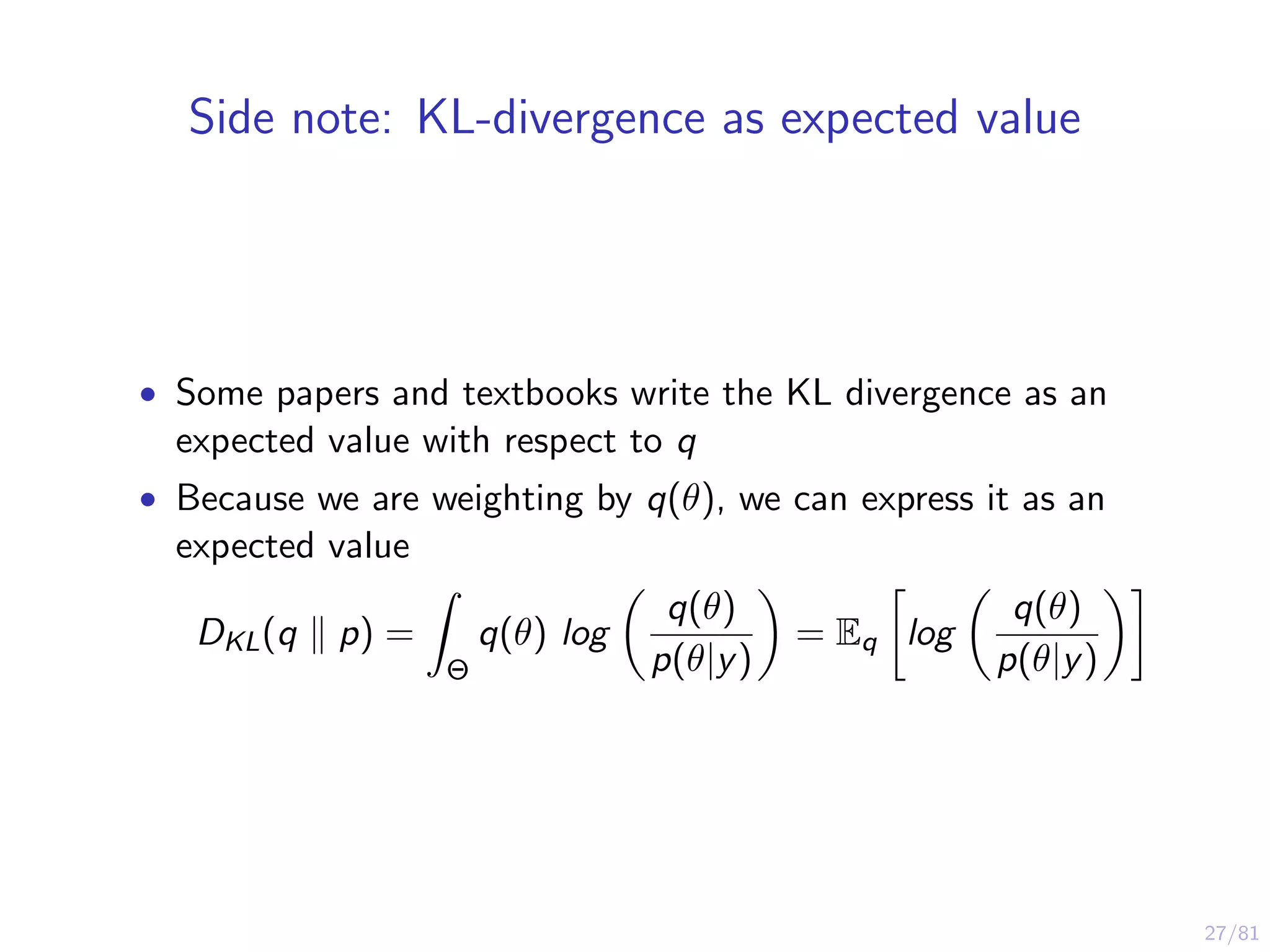
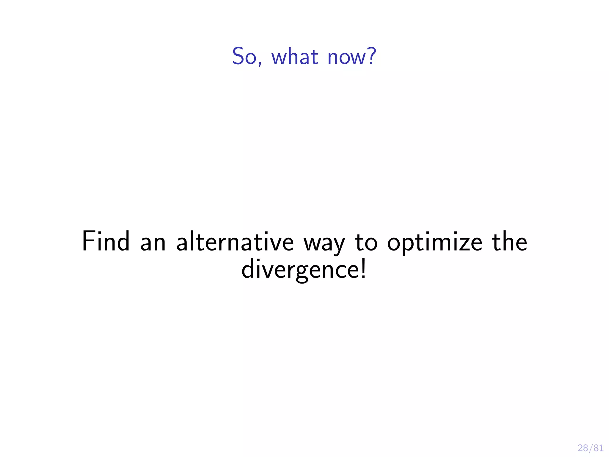
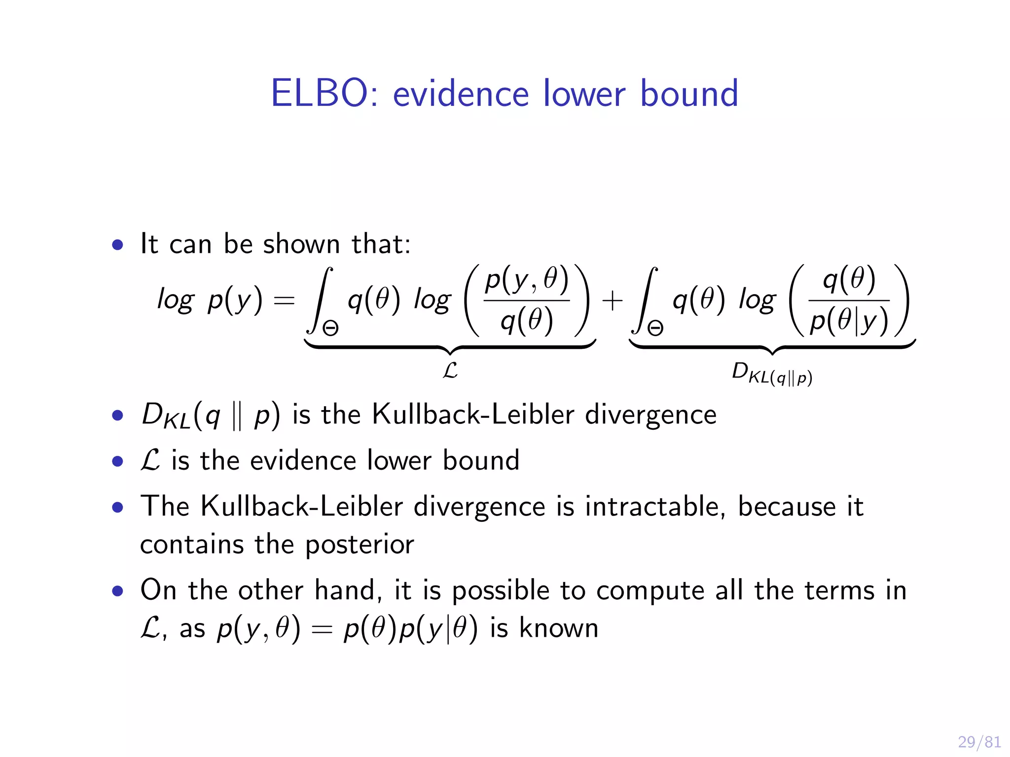
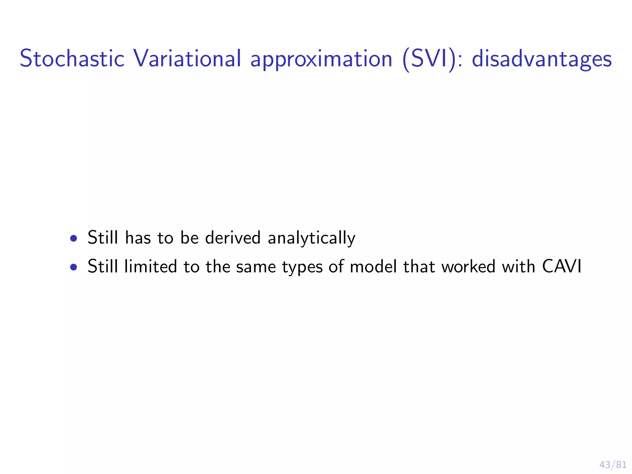
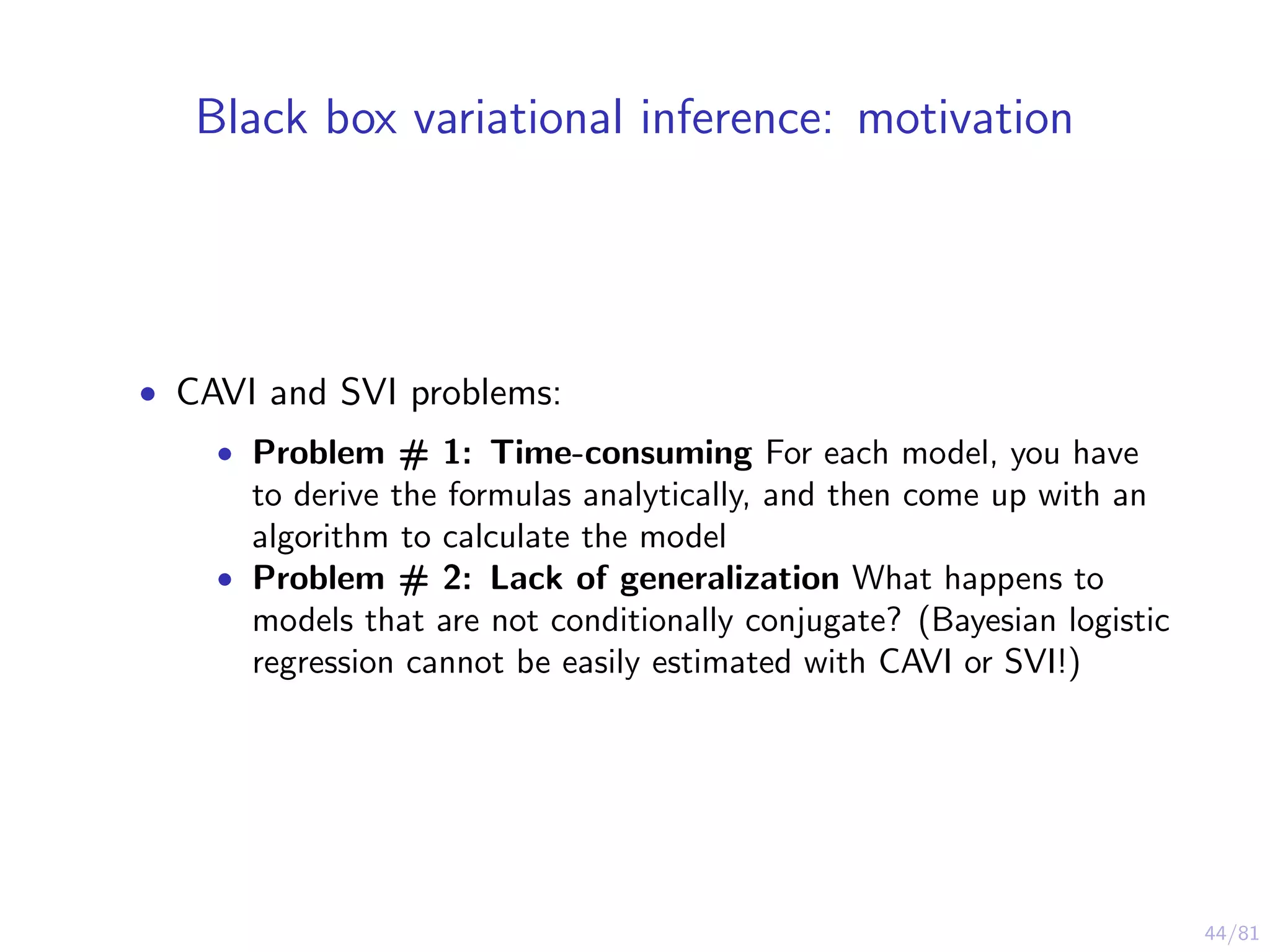
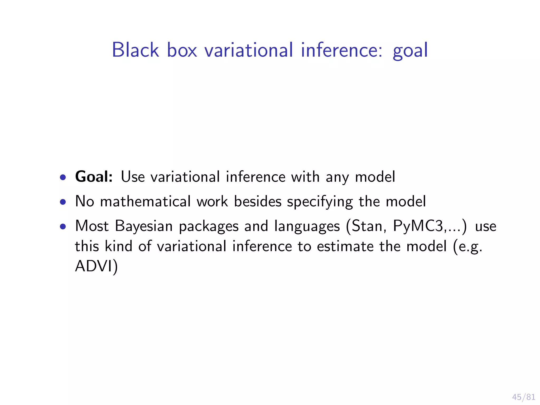
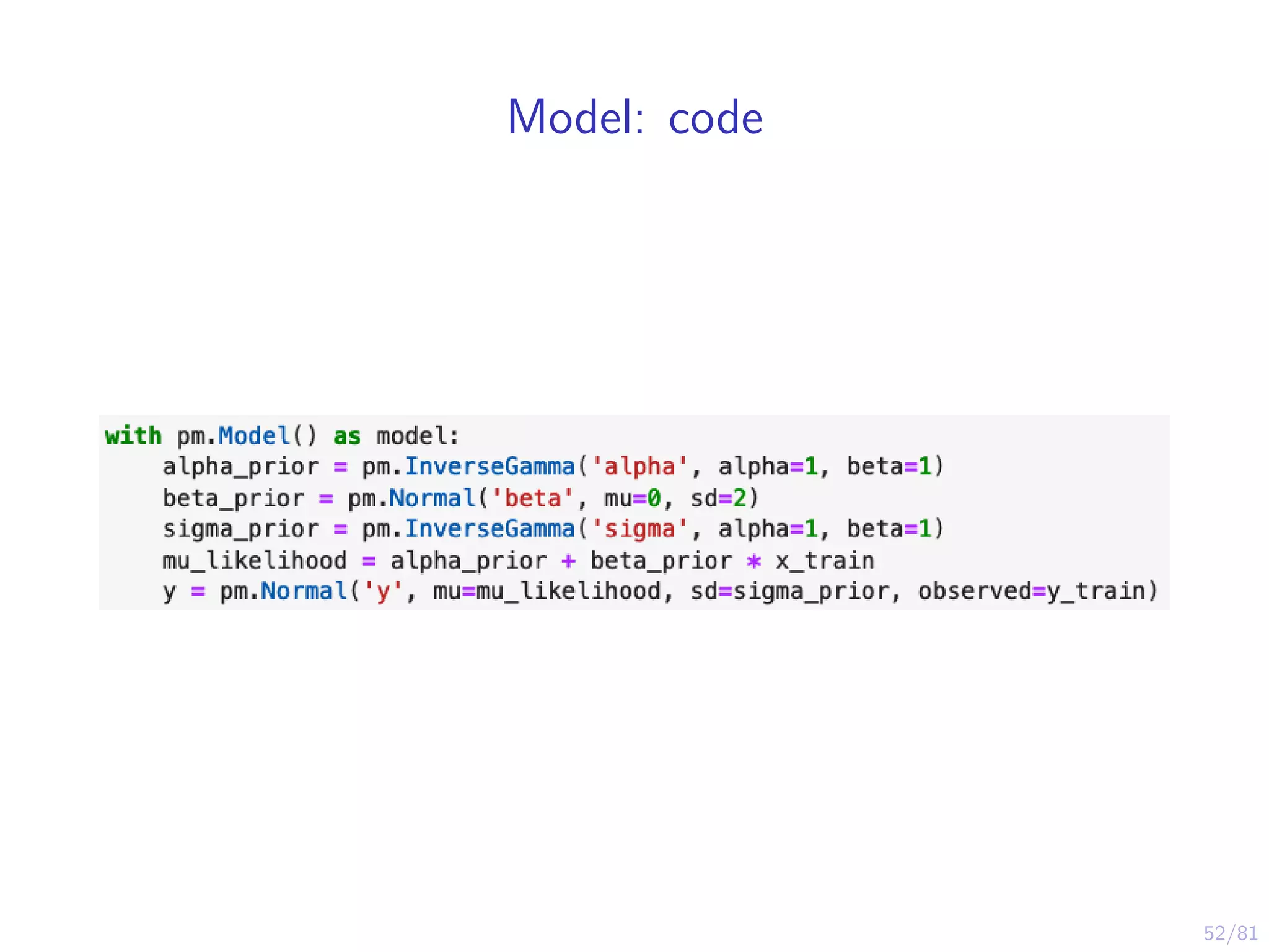
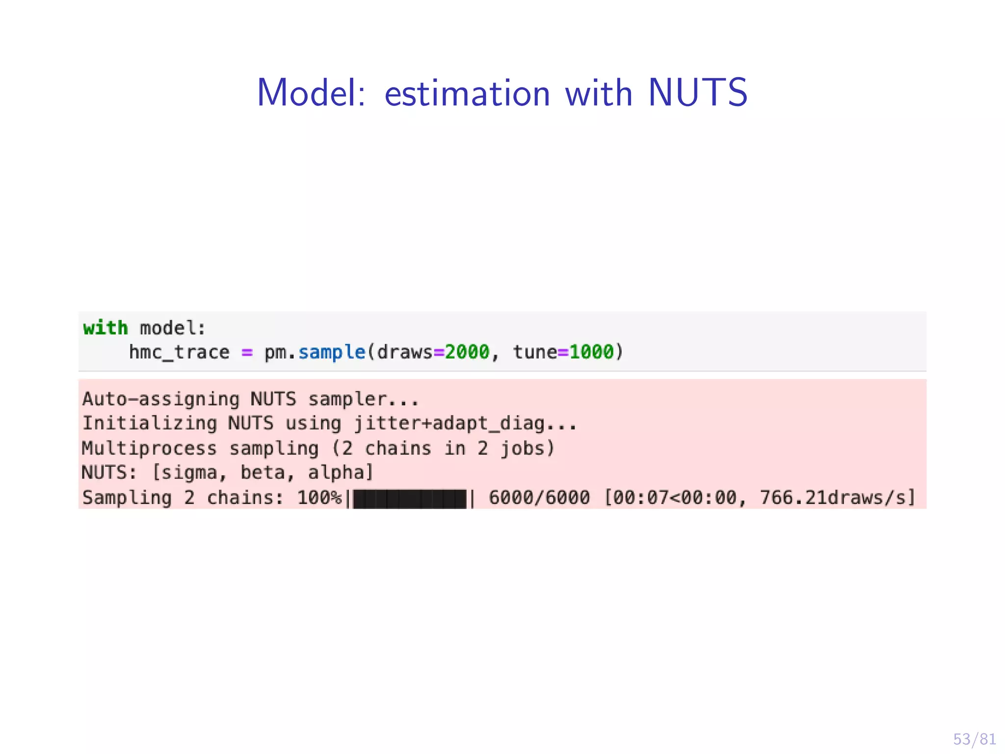
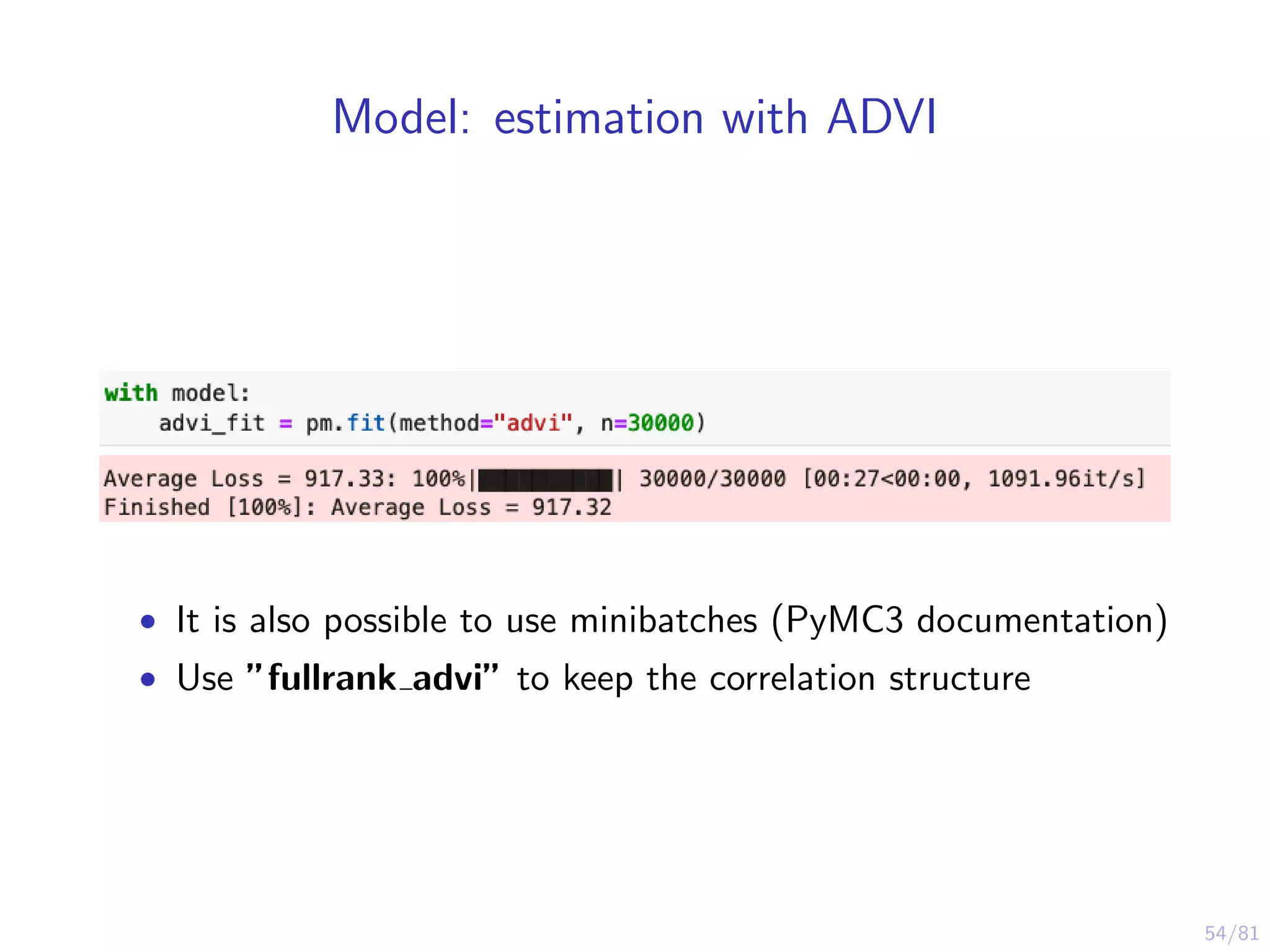
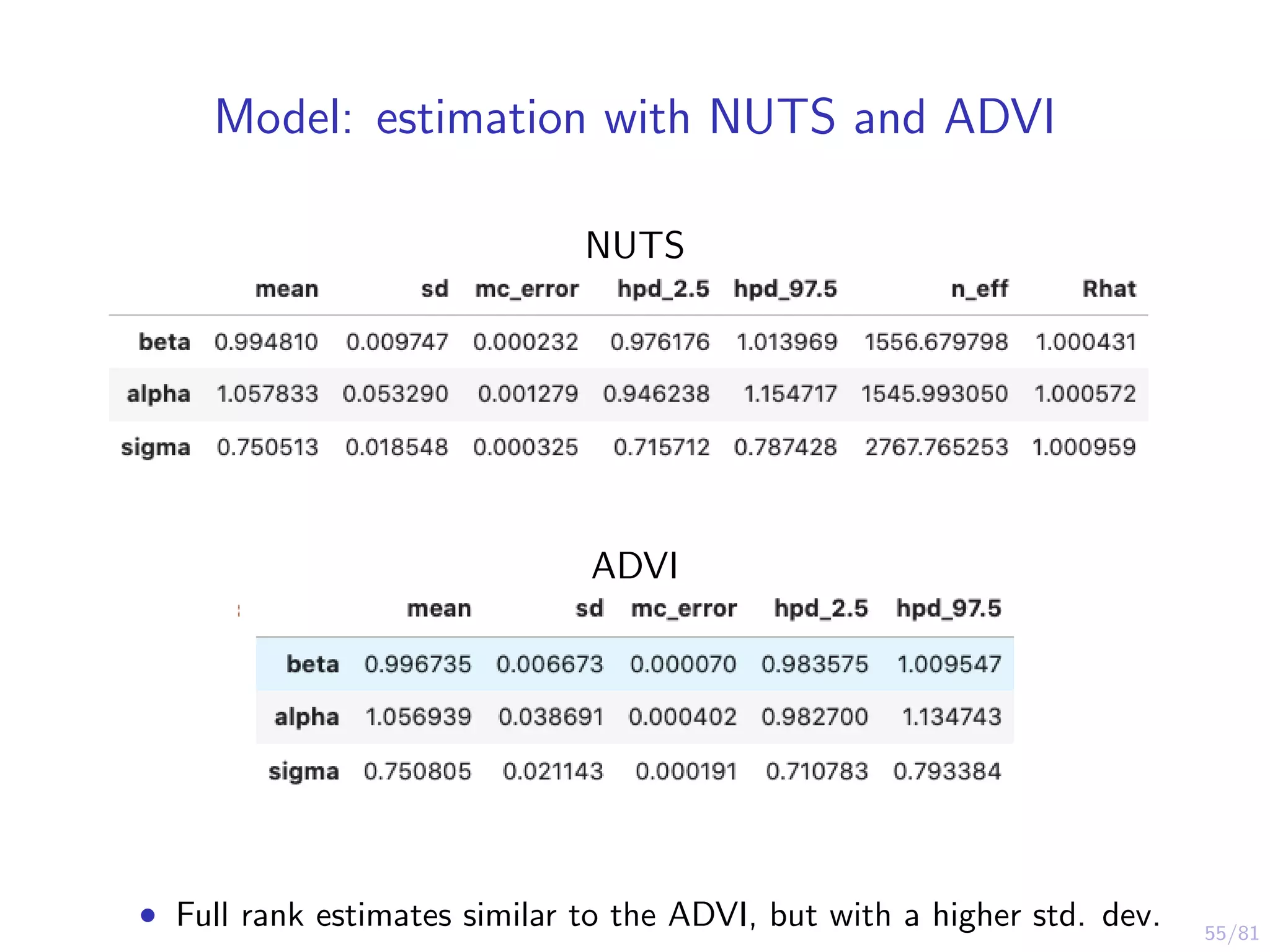
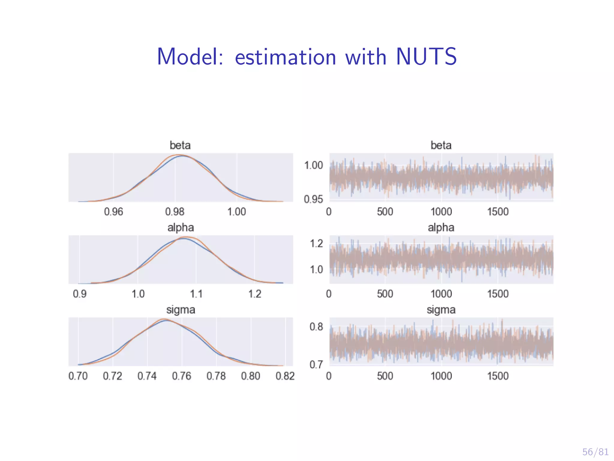
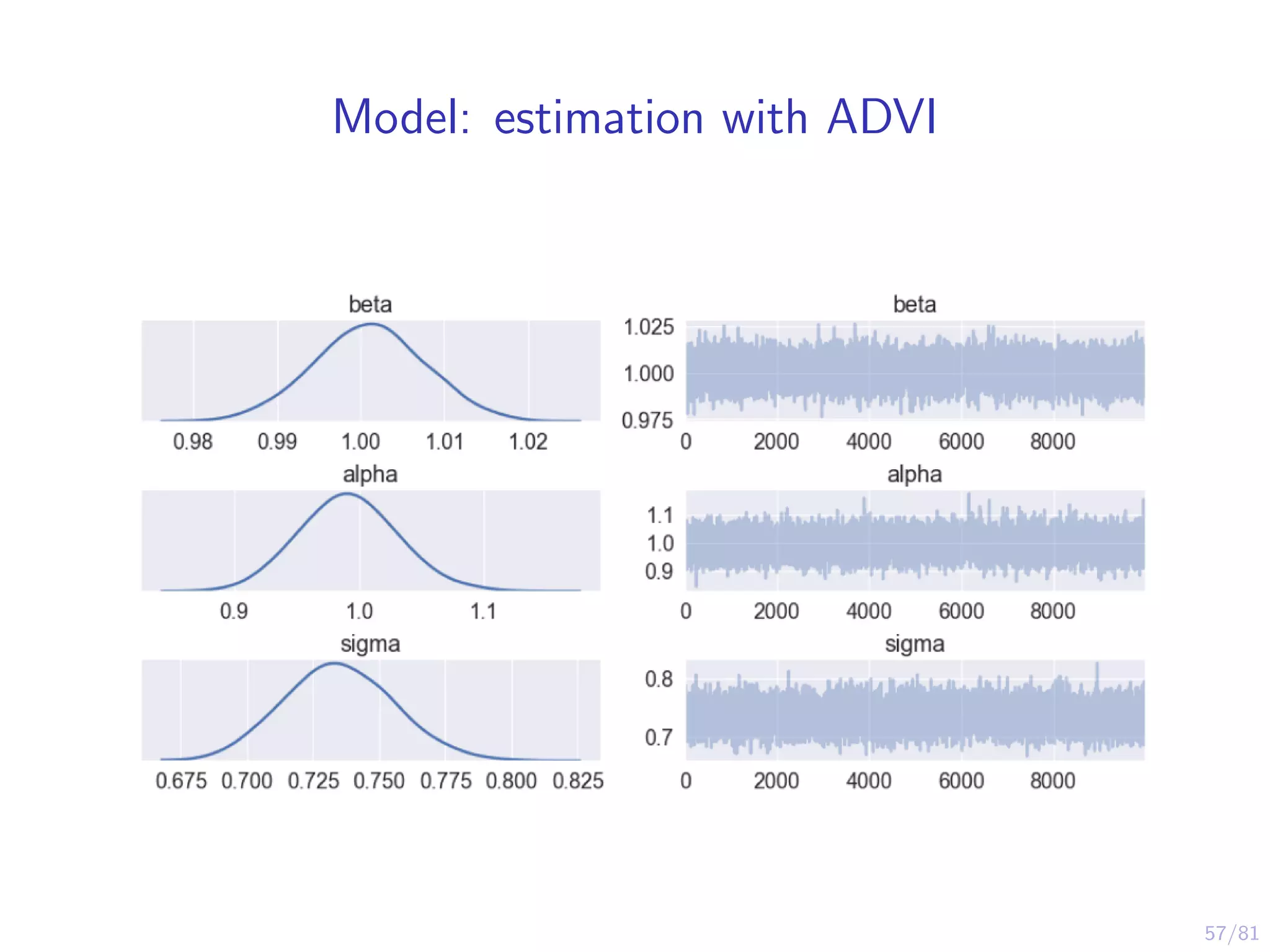
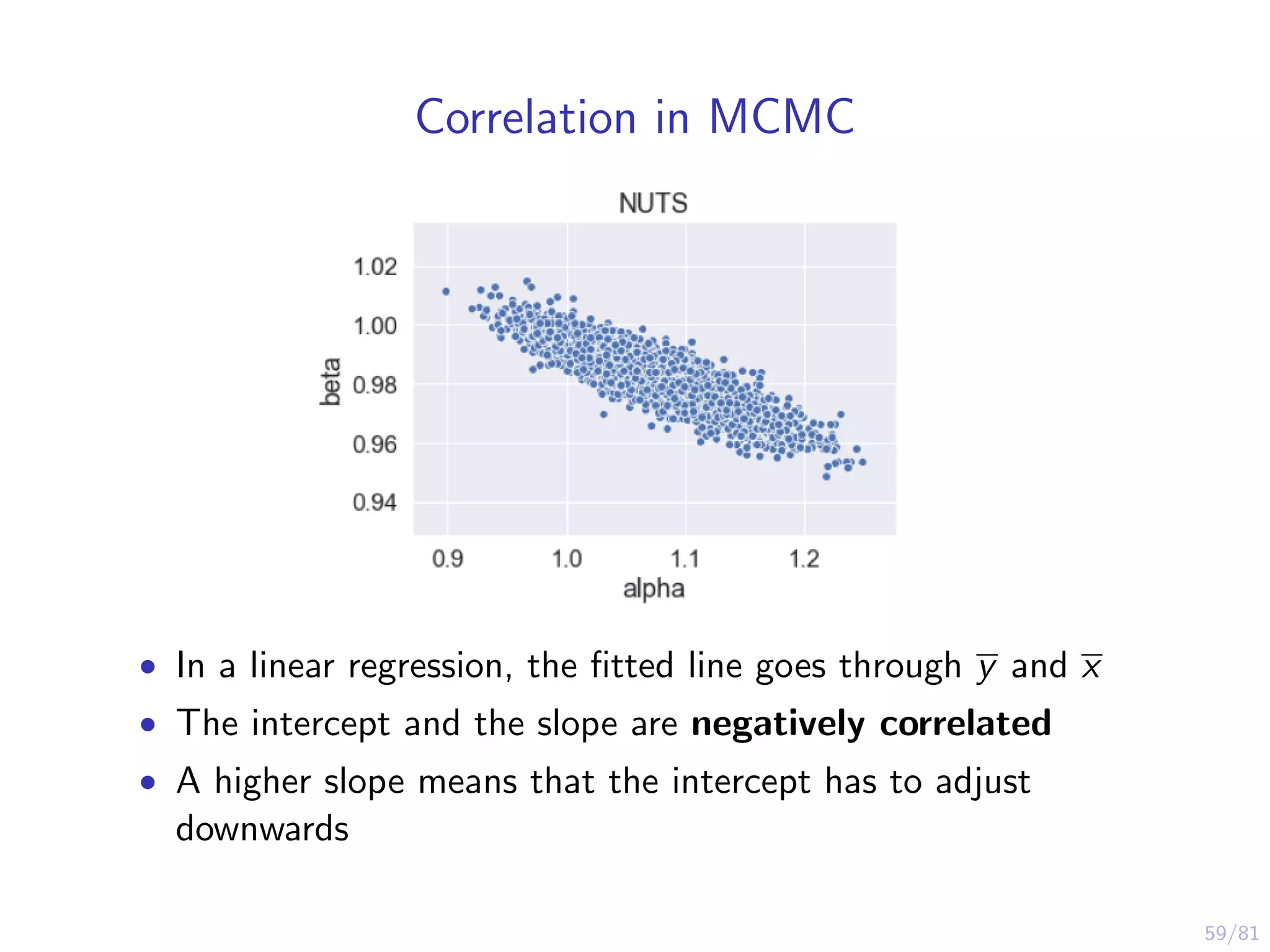
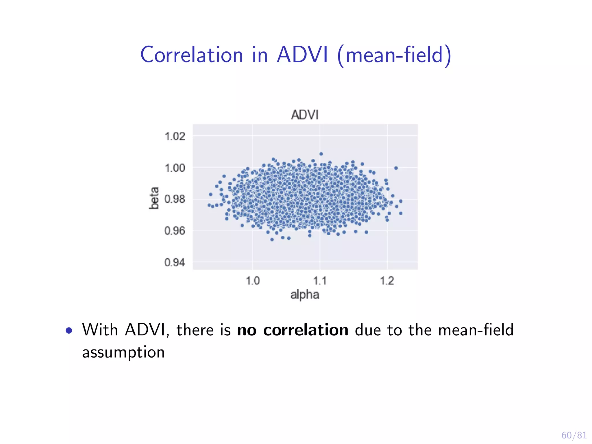
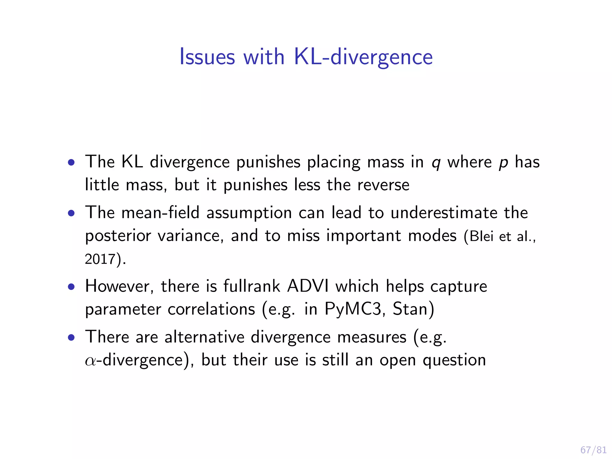
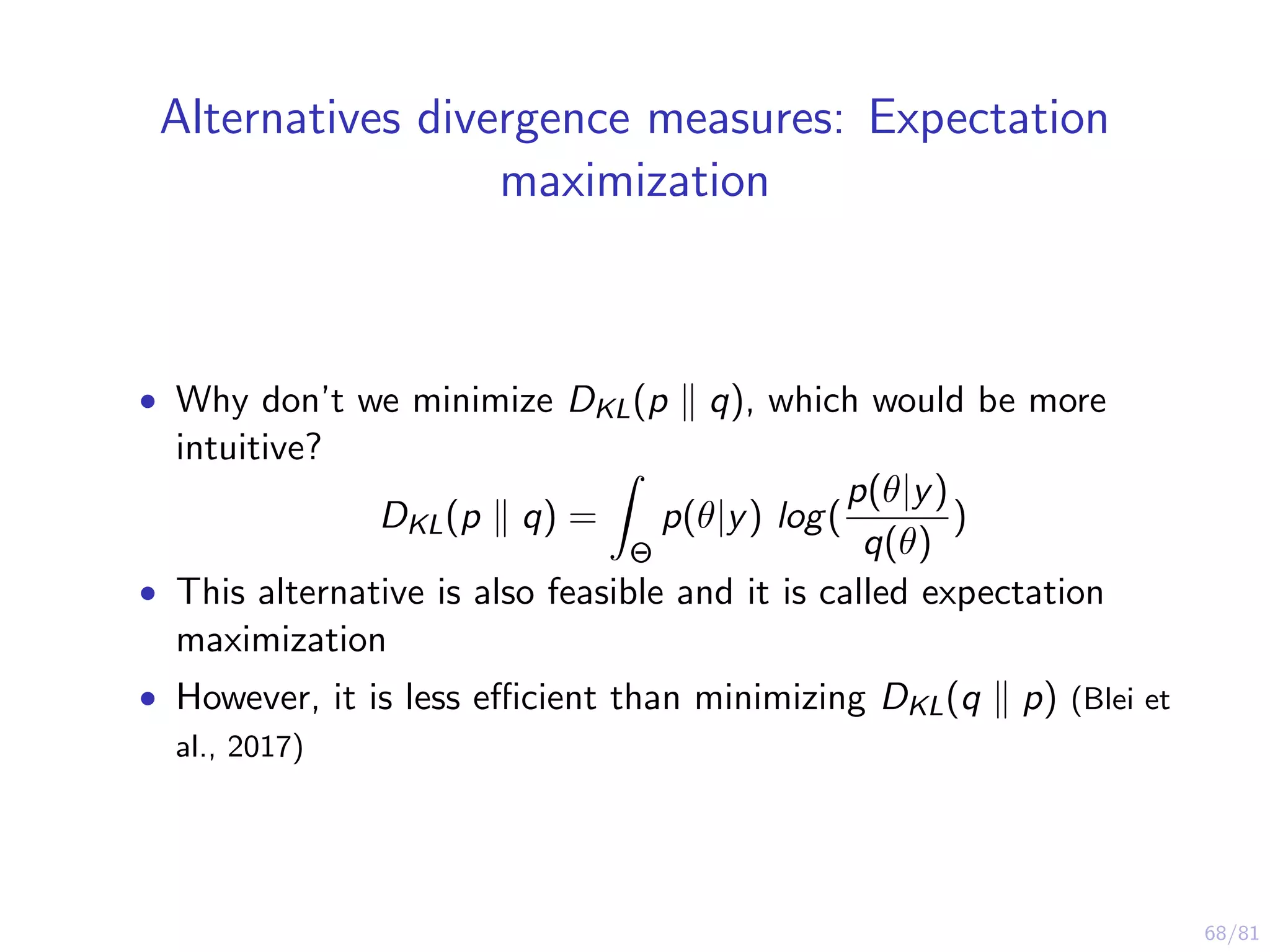
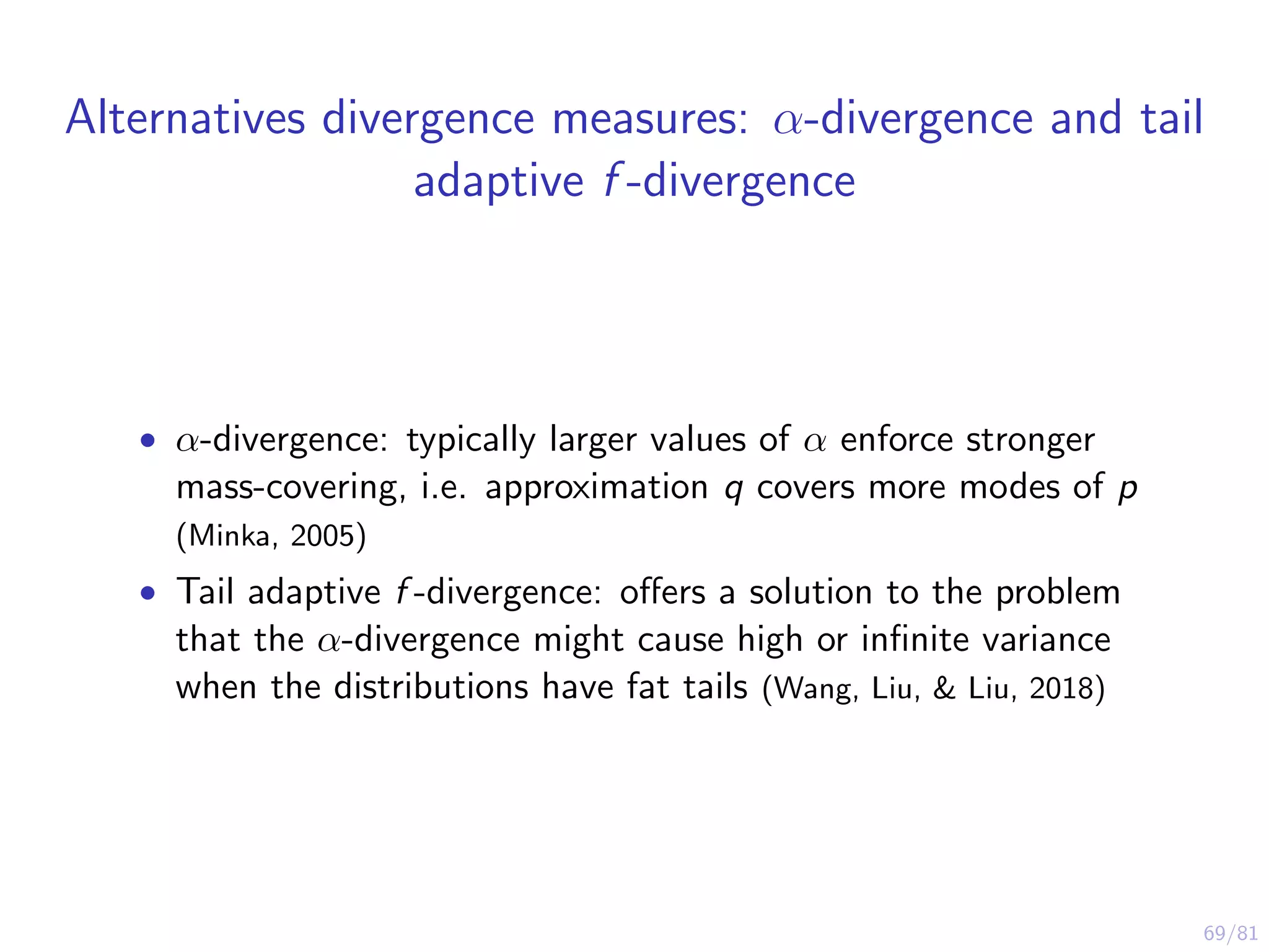
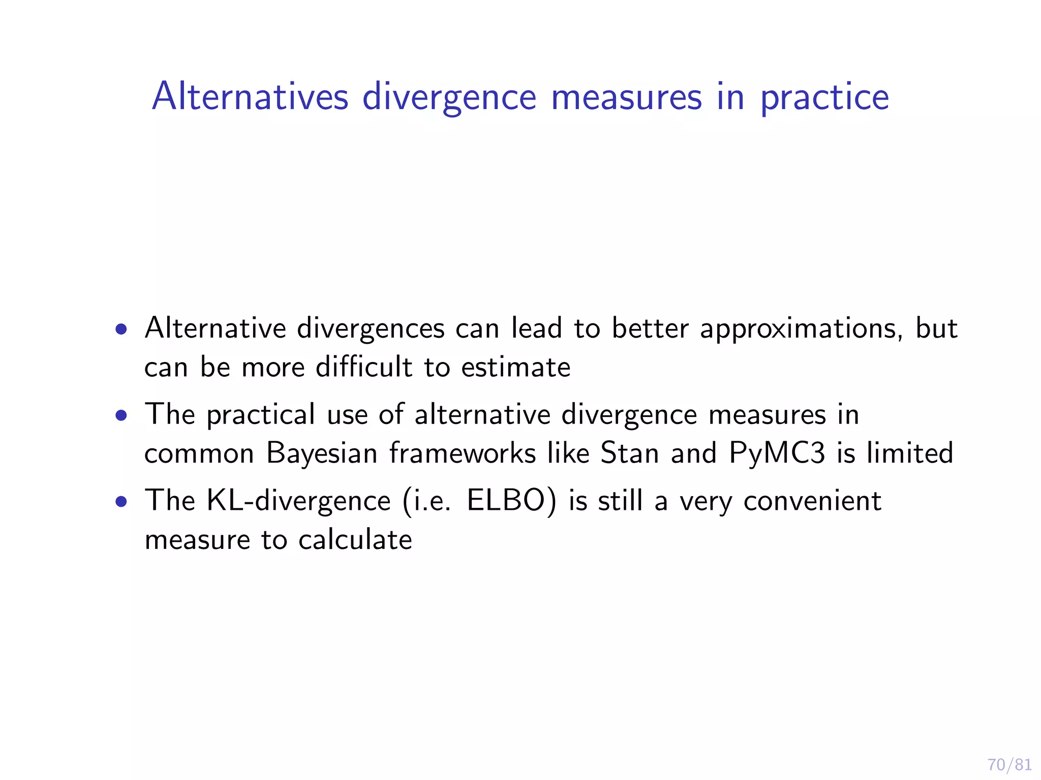
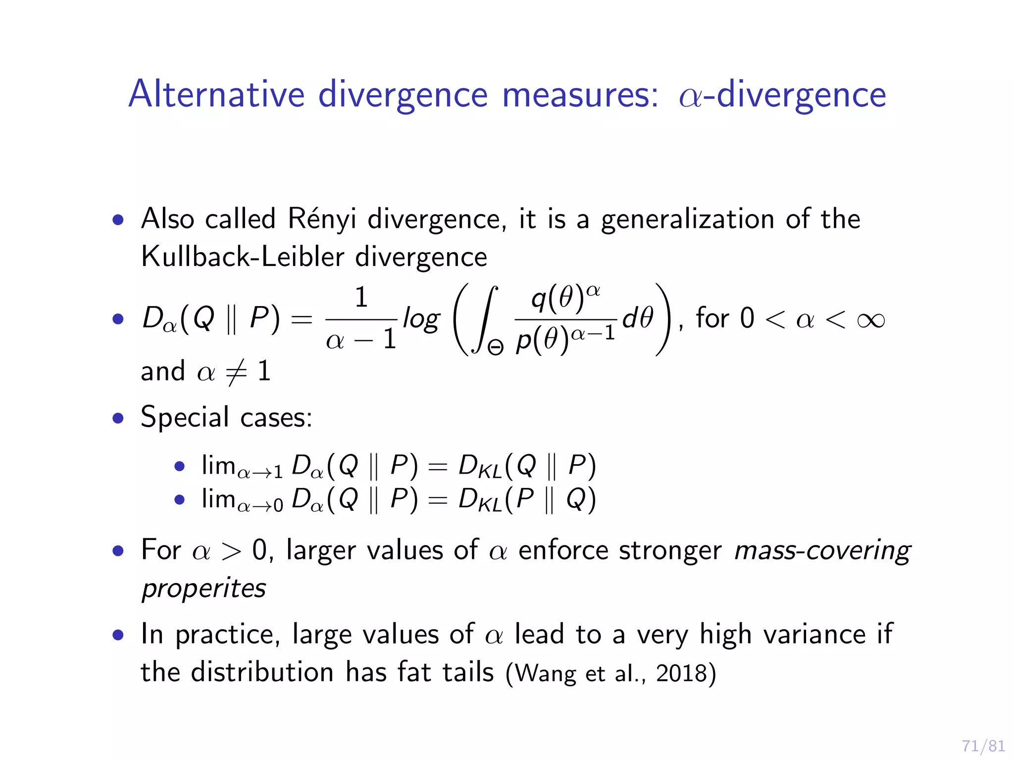
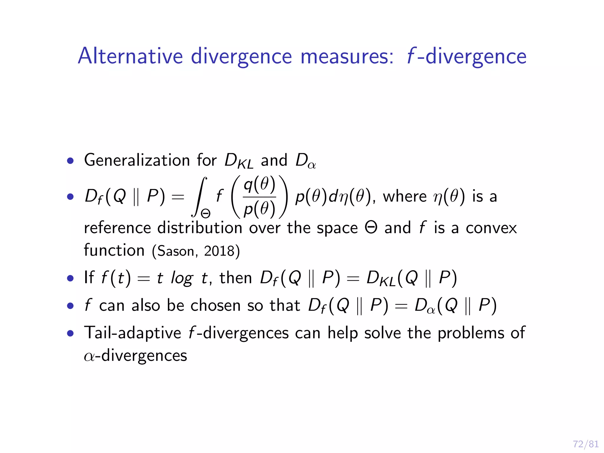
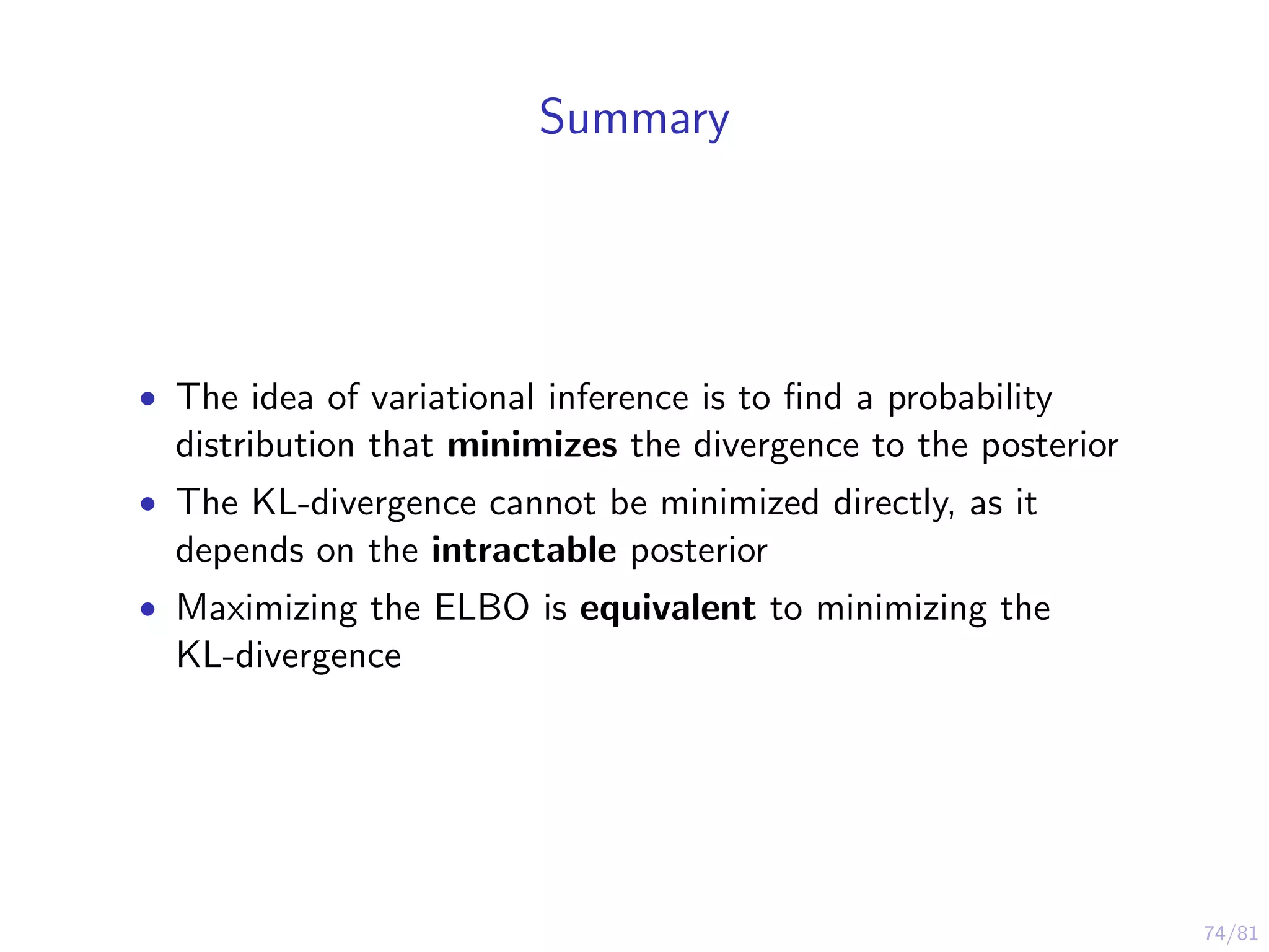
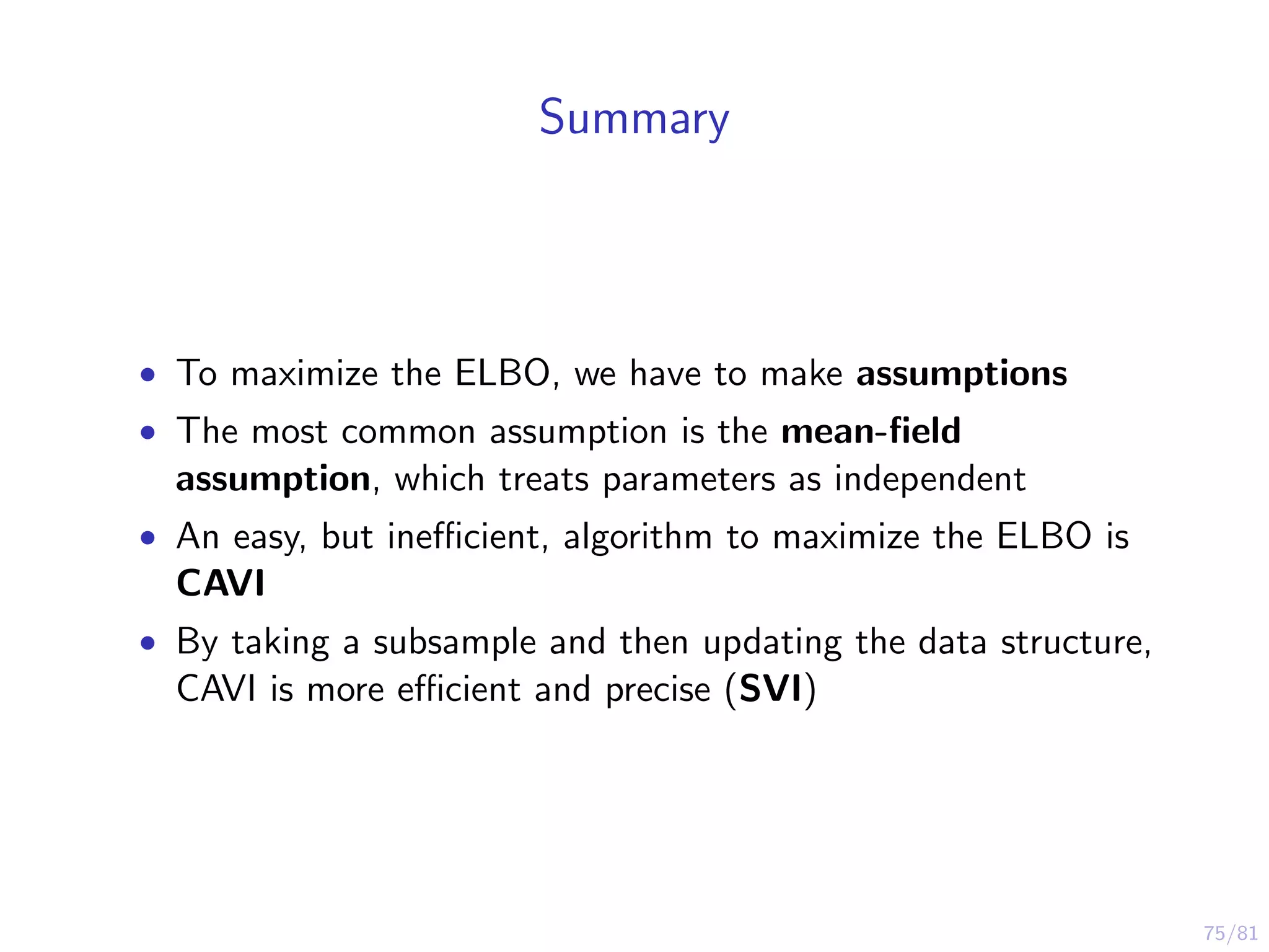
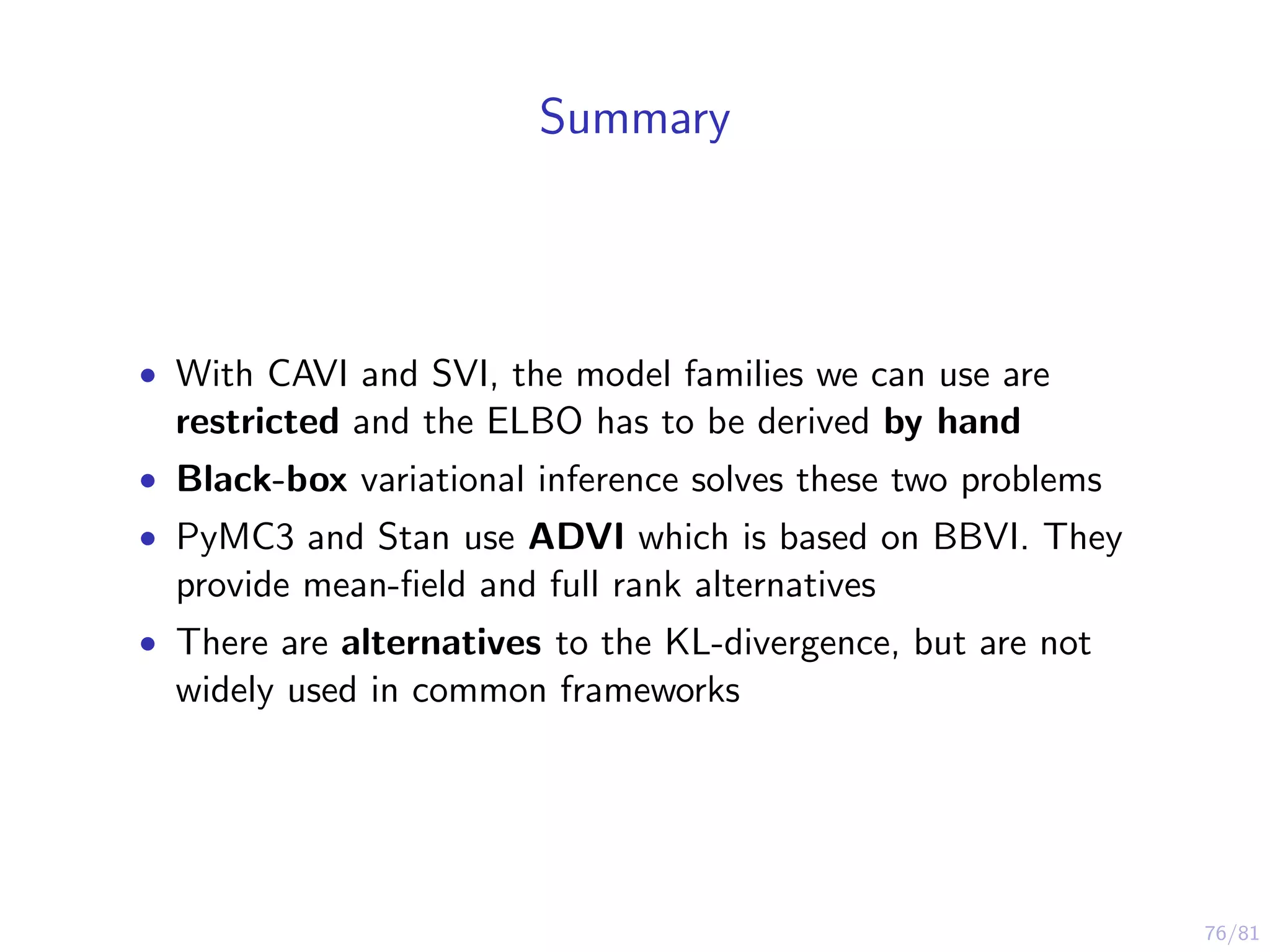
Variational Bayes:
A Gentle Introduction
Flavio Mejia Morelli
December 3, 2019
2/81
About me
• Flavio, from Bogot´a (Colombia)
• Education: MSc. Statistics at Humboldt University Berlin
• Work: statistical consulting unit of the Free University of
Berlin fu:stat
3/81
About this talk
• Basic knowledge of probability theory
• Basic knowledge of Bayesian statistics
• Focus on intuition, from a learner’s perspective
• However, Bayesian computation is still very technical
• Feel free to ask questions during the talk!
• For the material, check @ flaviomorelli on Twitter
4/81
Contents
1 What is variational Bayes?
2 Divergence between distributions
3 Estimating variational approximations
4 Example with PyMC3
5 Evaluating variational approximations
6 Alternative distance measures
7 Summary
5/81
Contents
1 What is variational Bayes?
2 Divergence between distributions
3 Estimating variational approximations
4 Example with PyMC3
5 Evaluating variational approximations
6 Alternative distance measures
7 Summary
6/81
Motivation: Why Variational Bayes?
• One of the main alternatives to MCMC
• Estimate different kinds of models much faster than MCMC
(usually at the expense of precision)
• However, variational inference is less well understood than
MCMC
7/81
Terminology: Bayes’ theorem
p(θ|y) =
p(θ, y)
p(y)
=
p(y|θ) · p(θ)
Θ p(y|θ) · p(θ)dθ
8/81
Terminology: Bayes’ theorem
p(θ|y) =
p(θ, y)
p(y)
=
p(y|θ) · p(θ)
Θ p(y|θ) · p(θ)dθ
• θ ∈ Θ: a parameter or vector of parameters (e.g. the
probability in a binomial distribution) in the parameter space
Θ
• y: data
• p(θ|y): posterior
• p(y|θ): likelihood function that captures how we are modeling
our data stochastically (e.g. y is a binomial variable)
• p(θ): prior knowledge about the parameters (e.g. a
probability can only be between 0 and 1)
9/81
Terminology: Bayes’ theorem
p(θ|y) =
p(θ, y)
p(y)
=
p(y|θ) · p(θ)
Θ p(y|θ) · p(θ)dθ
• p(y) = Θ p(y|θ) · p(θ)dθ: the marginal likelihood or evidence
• p(y) is a constant that normalizes the expression so that the
posterior integrates to one.
• Problem: p(y) is intractable even for very simple models,
and this makes it very hard to calculate the posterior
• Bayesian computation methods get around this intractability
by different means
10/81
MCMC and variational inference
• Markov Chain Monte Carlo (MCMC) is one of the most
common methods of estimating parameters in a Bayesian
model
• ”Little fly” takes samples from the parameter space to find
out how likely a given combination of parameters is
• Different approaches: Gibbs Sampler, Metropolis-Hastings,
Hamiltonian Monte Carlo, NUTS
• Pro: more Monte Carlo samples lead to a more accurate
estimate
• Con: slow and curse of dimensionality
11/81
MCMC and variational inference
• Variational inference turn the estimation of the posterior into
an optimization problem (i.e. maximize or minimize)
• Main idea: find another probability function that is easier to
work with than the posterior
• Minimize the difference between the new probability function
an the posterior
12/81
MCMC and variational inference
How do we measure the difference between
probability functions?
13/81
Contents
1 What is variational Bayes?
2 Divergence between distributions
3 Estimating variational approximations
4 Example with PyMC3
5 Evaluating variational approximations
6 Alternative distance measures
7 Summary
14/81
Difference between density functions
15/81
Difference between density functions
• Let p(x) and q(x) be two probability densities
• A naive approach for a given x:
q(x)
p(x)
16/81
Difference between density functions
• However, if we flip the terms we see that the absolute value of
this measure also changes: e.g. 0.3
0.1 = 3, but 0.1
0.3 = 1
3
• If we take the logarithm, the absolute value stays constant
after flipping the probabilities, only the sign changes:
log(q(x)
p(x) ) = −log(p(x)
q(x) )
17/81
Difference between density functions
• Assume that we are interested mainly on q(x)
• Use q(x) as a weight for the difference measure: q(x)log(q(x)
p(x) )
• When q(x) is low, the difference measure log(q(x)
p(x) ) does not
matter as much, as when q(x) is high!
18/81
Difference between density functions
• As a final step, we integrate over all the possible values of x
(or sum if the density is not continuous)
DKL = X q(x) log(q(x)
p(x) )dx
• DKL is called the Kullback-Leibler divergence of p from q
19/81
Kullback-Leibler Divergence
DKL(q p) = X q(x) log(q(x)
p(x) )dx
• Common measure for the divergence between two probability
densities
• The Kullback-Leibler divergence is not symmetric, and thus
is cannot be called a ”distance”: DKL(q p) = DKL(p q)
20/81
Kullback-Leibler Divergence
X q(x) log(q(x)
p(x) )dx = − X q(x) log(p(x)
q(x) )dx
• Note that if we flip the densities inside the logarithm, the
divergence does not change
• DKL ≥ 0 for any given probabilities. If DKL = 0 it means that
both probabilities are the same at each point
21/81
Examples of KL-Divergence: DKL(Q P)
22/81
Examples of KL-Divergence: : DKL(P Q)
23/81
Examples of KL-Divergence: : bimodal distribution
24/81
Examples of KL-Divergence: : bimodal distribution lower
variance
25/81
Variational approximation of the posterior
• Find a q∗(θ) which minimizes the KL divergence between q(θ)
and the posterior p(θ|y):
DKL(q p) =
Θ
q(θ) log(
q(θ)
p(θ|y)
)
• However, in order to calculate the KL divergence we would
have to know the posterior p(θ|y) which is intractable.
• We are back to square one...
26/81
Side note: What does ”variational” mean?
• The term ”variational” comes from variational calculus
• One of the main topics of calculus is optimization
• Optimization is usually done with respect to a variable.
• A common problem in economic is finding an optimum
quantity Q∗ that maximizes profit given a demand and a cost
function
• In contrast, variational calculus optimizes with respect to a
function. In our case, we are trying to find a q∗(θ) which
minimizes the Kullback-Leibler divergence
27/81
Side note: KL-divergence as expected value
• Some papers and textbooks write the KL divergence as an
expected value with respect to q
• Because we are weighting by q(θ), we can express it as an
expected value
DKL(q p) =
Θ
q(θ) log
q(θ)
p(θ|y)
= Eq log
q(θ)
p(θ|y)
28/81
So, what now?
Find an alternative way to optimize the
divergence!
29/81
ELBO: evidence lower bound
• It can be shown that:
log p(y) =
Θ
q(θ) log
p(y, θ)
q(θ)
L
+
Θ
q(θ) log
q(θ)
p(θ|y)
DKL(q p)
• DKL(q p) is the Kullback-Leibler divergence
• L is the evidence lower bound
• The Kullback-Leibler divergence is intractable, because it
contains the posterior
• On the other hand, it is possible to compute all the terms in
L, as p(y, θ) = p(θ)p(y|θ) is known
30/81
ELBO: derivation
log p(y) = log p(y) · 1 = log p(y)
Θ
q(θ)dθ
=
Θ
q(θ) log p(y)dθ =
Θ
q(θ) log
p(y, θ)
p(θ|y)
dθ
=
Θ
q(θ) log
p(y, θ)
p(θ|y)
·
q(θ)
q(θ)
dθ
=
Θ
q(θ) log
p(y, θ)
q(θ)
+
Θ
q(θ) log
q(θ)
p(θ|y)
Which can be written as (Ormerod & Wand, 2010):
log p(y) = L + DKL(q p)
31/81
ELBO: importance and optimization
• By rearranging we get:
L = log p(y) − DKL(q p)
• As DKL ≥ 0 ⇒ log p(y) ≥ L
• Therefore, L is the lower bound of the logarithm of the
evidence p(y)
• Hence the name evidence lower bound or ELBO for L
32/81
ELBO: importance and optimization
L = log p(y) − DKL(q p)
• Key idea: Maximizing the ELBO is equivalent to minimizing
the Kullback-Leibler divergence
• The idea of maximizing the ELBO is the basis of most
variational inference approaches
33/81
Contents
1 What is variational Bayes?
2 Divergence between distributions
3 Estimating variational approximations
4 Example with PyMC3
5 Evaluating variational approximations
6 Alternative distance measures
7 Summary
34/81
Making the ELBO tractable
• In theory, we could take any distribution q we like to
approximate the posterior
• However, there are usually restrictions on q to make the
problem more tractable
35/81
Making the ELBO tractable
• The most common restrictions are (Ormerod & Wand, 2010):
• Mean-field assumption: q(θ) factorizes into
M
i=1 qi (θi ) for
some partition {θ1, ..., θM }
• q comes from a parametric family of density functions
36/81
Mean-field assumption
q(θ) = M
i=1 qi (θi )
• E.g. normal distribution: p
µ
σ
= p(µ)p(σ)
• Note that the quality of the approximation depends on the
dependence between θi
• Example: given p(θ1, θ2|y), if θ1 and θ2 are highly dependent,
then the restriction q(θ1, θ2) = q1(θ1)q2(θ2) will cause a
degradation in the inference
37/81
Mean-field assumption
• The graphic shows a mean-field approximation of a
two-dimensional Gaussian posterior (Blei, Kucukelbir, & McAuliffe,
2017)
• Both distribution share the same mean, but the covariance
structure is different
38/81
Coordinate ascent variational inference: algorithm
1 Initialize q∗
2(θ2), ..., q∗
M(θM)
2 Cycle
q∗
1(θ1) =
exp{ E−θ1 log p(y, θ)}
exp{E−θ1 log p(y, θ)}dθ1
.
.
.
q∗
M(θM) =
exp{ E−θM
log p(y, θ)}
exp{E−θM
log p(y, θ)}dθM
Until the increase in the ELBO is negligible (Ormerod & Wand,
2010)
39/81
Coordinate ascent variational inference: key takeaways 1
• The algorithm is very inefficient, since is it use the complete
data set for each time it updates q∗
i (θi ), and then repeats
until ELBO converges
• This means CAVI cannot handle massive data
40/81
Coordinate ascent variational inference: key takeaways 2
• The ELBO or the optimal solution for q∗
i have to be
calculated by hand for each model
• There are good examples of the mathematical derivation
(with Python implementation) for a univariate Gaussian model
(Sia, 2019)
• Another example for the mathematical derivation of the
ELBO can be found in the original paper on Latent Dirichtlet
Allocation, a topic model algorithm (Blei, Ng, & Jordan, 2003)
41/81
Coordinate ascent variational inference: key takeaways 3
• This approach only works for conditionally conjugate
models like multilevel regression (e.g. linear, probit, Poisson),
matrix factorization (e.g. factor analysis, PCA),
mixed-membership models (e.g. LDA), etc. (Blei, 2017)
• There is a relation between the CAVI and Gibbs-Sampling
(Ormerod & Wand, 2010)
42/81
Stochastic Variational approximation (SVI)
• Based on stochastic approximation (Robbins & Monro, 1951)
• On each iteration: take a subsample of the data, infer the
local structure, update the global structure, repeat
• The gradient is noisy, but it is still doing the coordinate
ascent on the ELBO
• More efficient than CAVI, and more accurate results (Blei,
2017)
43/81
Stochastic Variational approximation (SVI): disadvantages
• Still has to be derived analytically
• Still limited to the same types of model that worked with CAVI
44/81
Black box variational inference: motivation
• CAVI and SVI problems:
• Problem # 1: Time-consuming For each model, you have
to derive the formulas analytically, and then come up with an
algorithm to calculate the model
• Problem # 2: Lack of generalization What happens to
models that are not conditionally conjugate? (Bayesian logistic
regression cannot be easily estimated with CAVI or SVI!)
45/81
Black box variational inference: goal
• Goal: Use variational inference with any model
• No mathematical work besides specifying the model
• Most Bayesian packages and languages (Stan, PyMC3,...) use
this kind of variational inference to estimate the model (e.g.
ADVI)
46/81
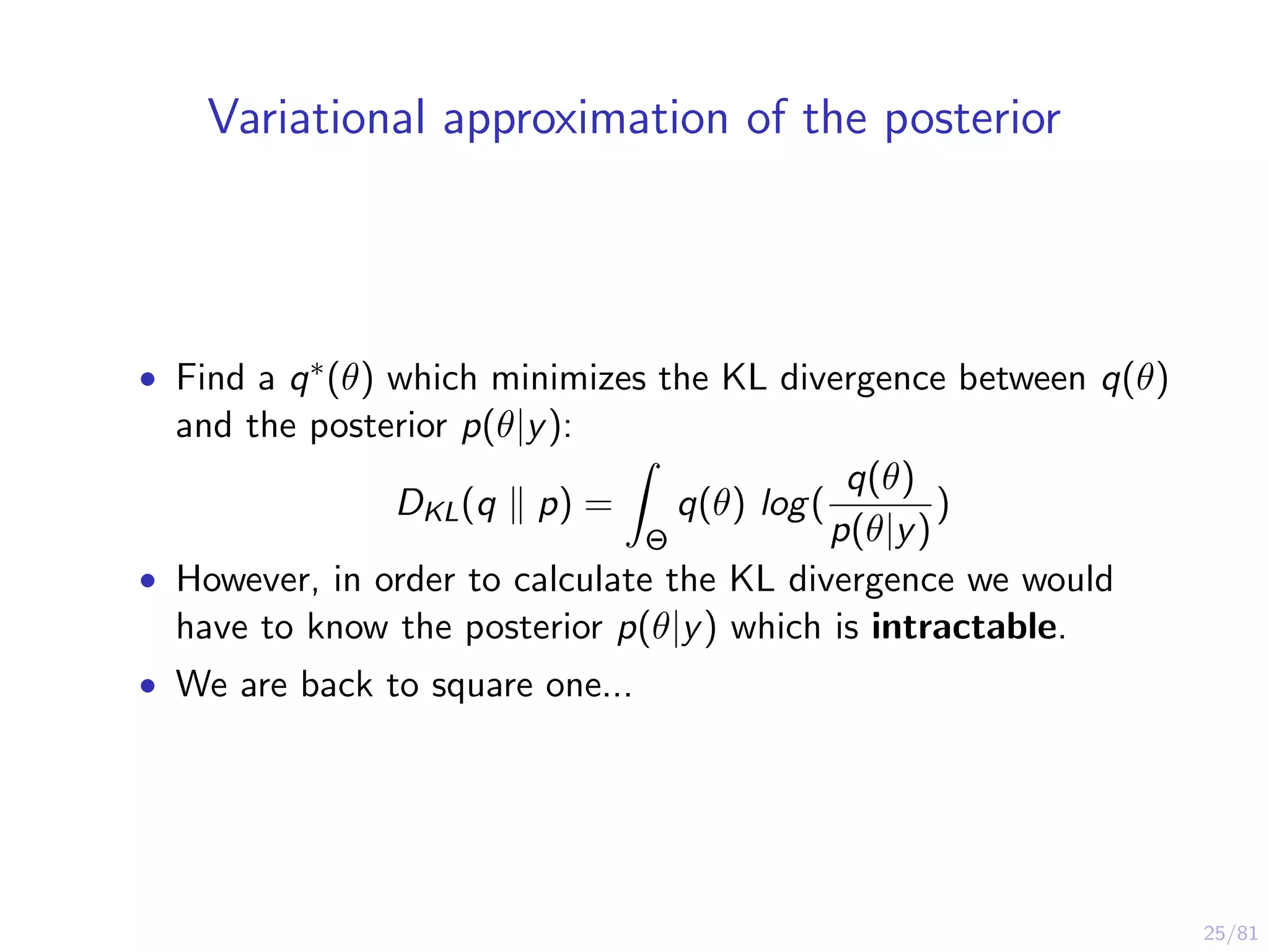
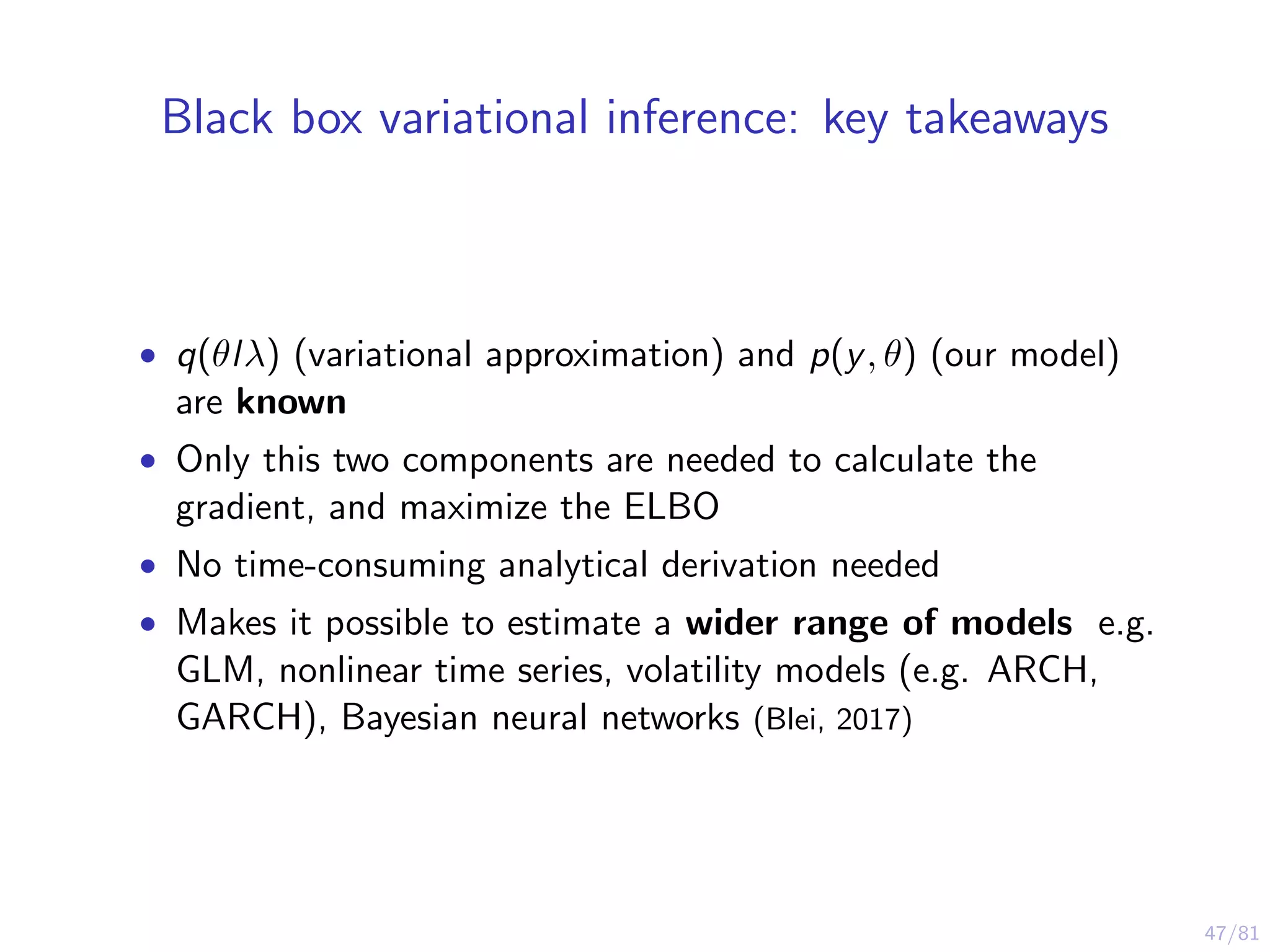
Black box variational inference: how does it work?
• Noisy gradient of the ELBO, λ is a hyperparameter (Ranganath,
Gerrish, & Blei, 2014):
λL = Eq[( λlog q(θ|λ))(log p(y, θ) − log q(θ|λ))]
• q(θ|λ) is from the variational families and can be stored in a
library
• p(y, θ) = p(θ)p(y|θ) is equivalent to writing down the model
• Black box criteria:
• Sample from q(θ|λ) (Monte Carlo)
• Evaluate λlog q(θ|λ)
• Evaluate log p(y, θ)
47/81
Black box variational inference: key takeaways
• q(θlλ) (variational approximation) and p(y, θ) (our model)
are known
• Only this two components are needed to calculate the
gradient, and maximize the ELBO
• No time-consuming analytical derivation needed
• Makes it possible to estimate a wider range of models e.g.
GLM, nonlinear time series, volatility models (e.g. ARCH,
GARCH), Bayesian neural networks (Blei, 2017)
48/81
Contents
1 What is variational Bayes?
2 Divergence between distributions
3 Estimating variational approximations
4 Example with PyMC3
5 Evaluating variational approximations
6 Alternative distance measures
7 Summary
49/81
Model: univariate linear regression
y = α + βx
y ∼ N(α + βx, σ)
α ∼ G−1(1, 1)
β ∼ N(0, 2)
σ ∼ G−1(1, 1)
• Note that the normal distribution is parametrized with the
standard deviation
• This examples is based on (Ioannides, 2018)
50/81
Model: true parameters
• The data is generated by simulation
• True parameters:
α = 1
β = 1
σ = 0.75
51/81
Model: simulated data
52/81
Model: code
53/81
Model: estimation with NUTS
54/81
Model: estimation with ADVI
• It is also possible to use minibatches (PyMC3 documentation)
• Use ”fullrank advi” to keep the correlation structure
55/81
Model: estimation with NUTS and ADVI
NUTS
ADVI
• Full rank estimates similar to the ADVI, but with a higher std. dev.
56/81
Model: estimation with NUTS
57/81
Model: estimation with ADVI
58/81
Model: maximizing the ELBO
59/81
Correlation in MCMC
• In a linear regression, the fitted line goes through y and x
• The intercept and the slope are negatively correlated
• A higher slope means that the intercept has to adjust
downwards
60/81
Correlation in ADVI (mean-field)
• With ADVI, there is no correlation due to the mean-field
assumption
61/81
Correlation in Full Rank ADVI
• Full rank ADVI takes into account the covariance structure
of the model
• However, it can take longer to estimate
62/81
Contents
1 What is variational Bayes?
2 Divergence between distributions
3 Estimating variational approximations
4 Example with PyMC3
5 Evaluating variational approximations
6 Alternative distance measures
7 Summary
63/81
Evaluating variational inference
• It can be challenging to discover problems with posterior
approximation (Yao, Vehtari, Simpson, & Gelman, 2018)
• Variational inference approaches come with few theoretical
guarantees
• It is difficult to assess the quality of the approximation
64/81
Evaluating variational inference
• Usual problems (Blei et al., 2017):
• Slow ELBO convergence
• The inability of the approximation family to capture the true
posterior
• The mean-field assumption makes it difficult to calculate
posterior correlation
• The asymmetry of the true distribution
• KL divergence under-penalizes approximations with too light
tails
65/81
Diagnostics in common Bayesian frameworks
• Both Stan and PyMC3 use ADVI (Kucukelbir, Tran, Ranganath,
Gelman, & Blei, 2017), which is related to Black Box variational
inference
• Both frameworks have convergence diagnostics (in Stan
there is still an open pull request to impolement all the
diagnostics from the Yao et al. paper)
66/81
Contents
1 What is variational Bayes?
2 Divergence between distributions
3 Estimating variational approximations
4 Example with PyMC3
5 Evaluating variational approximations
6 Alternative distance measures
7 Summary
67/81
Issues with KL-divergence
• The KL divergence punishes placing mass in q where p has
little mass, but it punishes less the reverse
• The mean-field assumption can lead to underestimate the
posterior variance, and to miss important modes (Blei et al.,
2017).
• However, there is fullrank ADVI which helps capture
parameter correlations (e.g. in PyMC3, Stan)
• There are alternative divergence measures (e.g.
α-divergence), but their use is still an open question
68/81
Alternatives divergence measures: Expectation
maximization
• Why don’t we minimize DKL(p q), which would be more
intuitive?
DKL(p q) =
Θ
p(θ|y) log(
p(θ|y)
q(θ)
)
• This alternative is also feasible and it is called expectation
maximization
• However, it is less efficient than minimizing DKL(q p) (Blei et
al., 2017)
69/81
Alternatives divergence measures: α-divergence and tail
adaptive f -divergence
• α-divergence: typically larger values of α enforce stronger
mass-covering, i.e. approximation q covers more modes of p
(Minka, 2005)
• Tail adaptive f -divergence: offers a solution to the problem
that the α-divergence might cause high or infinite variance
when the distributions have fat tails (Wang, Liu, & Liu, 2018)
70/81
Alternatives divergence measures in practice
• Alternative divergences can lead to better approximations, but
can be more difficult to estimate
• The practical use of alternative divergence measures in
common Bayesian frameworks like Stan and PyMC3 is limited
• The KL-divergence (i.e. ELBO) is still a very convenient
measure to calculate
71/81
Alternative divergence measures: α-divergence
• Also called R´enyi divergence, it is a generalization of the
Kullback-Leibler divergence
• Dα(Q P) =
1
α − 1
log
Θ
q(θ)α
p(θ)α−1
dθ , for 0 < α < ∞
and α = 1
• Special cases:
• limα→1 Dα(Q P) = DKL(Q P)
• limα→0 Dα(Q P) = DKL(P Q)
• For α > 0, larger values of α enforce stronger mass-covering
properites
• In practice, large values of α lead to a very high variance if
the distribution has fat tails (Wang et al., 2018)
72/81
Alternative divergence measures: f -divergence
• Generalization for DKL and Dα
• Df (Q P) =
Θ
f
q(θ)
p(θ)
p(θ)dη(θ), where η(θ) is a
reference distribution over the space Θ and f is a convex
function (Sason, 2018)
• If f (t) = t log t, then Df (Q P) = DKL(Q P)
• f can also be chosen so that Df (Q P) = Dα(Q P)
• Tail-adaptive f -divergences can help solve the problems of
α-divergences
73/81
Contents
1 What is variational Bayes?
2 Divergence between distributions
3 Estimating variational approximations
4 Example with PyMC3
5 Evaluating variational approximations
6 Alternative distance measures
7 Summary
74/81
Summary
• The idea of variational inference is to find a probability
distribution that minimizes the divergence to the posterior
• The KL-divergence cannot be minimized directly, as it
depends on the intractable posterior
• Maximizing the ELBO is equivalent to minimizing the
KL-divergence
75/81
Summary
• To maximize the ELBO, we have to make assumptions
• The most common assumption is the mean-field
assumption, which treats parameters as independent
• An easy, but inefficient, algorithm to maximize the ELBO is
CAVI
• By taking a subsample and then updating the data structure,
CAVI is more efficient and precise (SVI)
76/81
Summary
• With CAVI and SVI, the model families we can use are
restricted and the ELBO has to be derived by hand
• Black-box variational inference solves these two problems
• PyMC3 and Stan use ADVI which is based on BBVI. They
provide mean-field and full rank alternatives
• There are alternatives to the KL-divergence, but are not
widely used in common frameworks
77/81
Summary
What do I really need to know about
variational inference?
78/81
Twitter: @ flaviomorelli
GitHub: @flaviomorelli
LinkedIn: Flavio Morelli
Email: flavio.morelli@fu-berlin.de
79/81
Bibliography I
Blei, D. M. (2017). Variational Inference: Foundations and
Innovations. Retrieved 2019-11-30, from
https://youtu.be/Dv86zdWjJKQ
Blei, D. M., Kucukelbir, A., & McAuliffe, J. D. (2017). Variational
Inference: A Review for Statisticians. Journal of the
American Statistical Association, 112(518), 859–877.
Blei, D. M., Ng, A. Y., & Jordan, M. I. (2003). Latent Dirichlet
Allocation. Journal of Machine Learning Research, 3,
993–1022.
Ioannides, A. (2018). Regression in PYMC3 using MCMC &
VariationalInference. Retrieved 2019-11-25, from https://
alexioannides.com/2018/11/07/bayesian-regression
-in-pymc3-using-mcmc-variational-inference
80/81
Bibliography II
Kucukelbir, A., Tran, D., Ranganath, R., Gelman, A., & Blei,
D. M. (2017). Automatic Differentiation Variational
Inference. Journal of Machine Learning Research, 18(14),
1–45.
Minka, T. (2005). Divergence measures and message passing
(Tech. Rep. No. MSR-TR-2005-173). Microsoft Research.
Ormerod, J. T., & Wand, M. P. (2010). Explaining Variational
Approximations. The American Statistician, 64(2), 140–153.
Ranganath, R., Gerrish, S., & Blei, D. M. (2014). Black Box
Variational Inference. In Proceedings of Artificial Intelligence
and Statistics.
Robbins, H., & Monro, S. (1951). A Stochastic Approximation
Method. The Annals of Mathematical Statistics, 22(3),
400–407.
Sason, I. (2018). On f-Divergences: Integral Representations,
Local Behavior, and Inequalities. Entropy, 20(5), 383.
81/81
Bibliography III
Sia, X. Y. S. (2019). Coordinate Ascent Mean-field Variational
Inference (Univariate Gaussian Example). Retrieved
2019-11-20, from https://suzyahyah.github.io/
bayesian%20inference/machine%20learning/
variational%20inference/2019/03/20/CAVI.html
Wang, D., Liu, H., & Liu, Q. (2018). Variational Inference with
Tail-adaptive f-Divergence. In Advances in Neural
Information Processing Systems.
Yao, Y., Vehtari, A., Simpson, D., & Gelman, A. (2018). Yes, but
Did It Work?: Evaluating Variational Inference. In
Proceedings of the 35th International Conference on
Machine Learning.

Variational Bayes: A Gentle Introduction

  • 1.
    Variational Bayes: A GentleIntroduction Flavio Mejia Morelli December 3, 2019
  • 2.
    2/81 About me • Flavio,from Bogot´a (Colombia) • Education: MSc. Statistics at Humboldt University Berlin • Work: statistical consulting unit of the Free University of Berlin fu:stat
  • 3.
    3/81 About this talk •Basic knowledge of probability theory • Basic knowledge of Bayesian statistics • Focus on intuition, from a learner’s perspective • However, Bayesian computation is still very technical • Feel free to ask questions during the talk! • For the material, check @ flaviomorelli on Twitter
  • 4.
    4/81 Contents 1 What isvariational Bayes? 2 Divergence between distributions 3 Estimating variational approximations 4 Example with PyMC3 5 Evaluating variational approximations 6 Alternative distance measures 7 Summary
  • 5.
    5/81 Contents 1 What isvariational Bayes? 2 Divergence between distributions 3 Estimating variational approximations 4 Example with PyMC3 5 Evaluating variational approximations 6 Alternative distance measures 7 Summary
  • 6.
    6/81 Motivation: Why VariationalBayes? • One of the main alternatives to MCMC • Estimate different kinds of models much faster than MCMC (usually at the expense of precision) • However, variational inference is less well understood than MCMC
  • 7.
    7/81 Terminology: Bayes’ theorem p(θ|y)= p(θ, y) p(y) = p(y|θ) · p(θ) Θ p(y|θ) · p(θ)dθ
  • 8.
    8/81 Terminology: Bayes’ theorem p(θ|y)= p(θ, y) p(y) = p(y|θ) · p(θ) Θ p(y|θ) · p(θ)dθ • θ ∈ Θ: a parameter or vector of parameters (e.g. the probability in a binomial distribution) in the parameter space Θ • y: data • p(θ|y): posterior • p(y|θ): likelihood function that captures how we are modeling our data stochastically (e.g. y is a binomial variable) • p(θ): prior knowledge about the parameters (e.g. a probability can only be between 0 and 1)
  • 9.
    9/81 Terminology: Bayes’ theorem p(θ|y)= p(θ, y) p(y) = p(y|θ) · p(θ) Θ p(y|θ) · p(θ)dθ • p(y) = Θ p(y|θ) · p(θ)dθ: the marginal likelihood or evidence • p(y) is a constant that normalizes the expression so that the posterior integrates to one. • Problem: p(y) is intractable even for very simple models, and this makes it very hard to calculate the posterior • Bayesian computation methods get around this intractability by different means
  • 10.
    10/81 MCMC and variationalinference • Markov Chain Monte Carlo (MCMC) is one of the most common methods of estimating parameters in a Bayesian model • ”Little fly” takes samples from the parameter space to find out how likely a given combination of parameters is • Different approaches: Gibbs Sampler, Metropolis-Hastings, Hamiltonian Monte Carlo, NUTS • Pro: more Monte Carlo samples lead to a more accurate estimate • Con: slow and curse of dimensionality
  • 11.
    11/81 MCMC and variationalinference • Variational inference turn the estimation of the posterior into an optimization problem (i.e. maximize or minimize) • Main idea: find another probability function that is easier to work with than the posterior • Minimize the difference between the new probability function an the posterior
  • 12.
    12/81 MCMC and variationalinference How do we measure the difference between probability functions?
  • 13.
    13/81 Contents 1 What isvariational Bayes? 2 Divergence between distributions 3 Estimating variational approximations 4 Example with PyMC3 5 Evaluating variational approximations 6 Alternative distance measures 7 Summary
  • 14.
  • 15.
    15/81 Difference between densityfunctions • Let p(x) and q(x) be two probability densities • A naive approach for a given x: q(x) p(x)
  • 16.
    16/81 Difference between densityfunctions • However, if we flip the terms we see that the absolute value of this measure also changes: e.g. 0.3 0.1 = 3, but 0.1 0.3 = 1 3 • If we take the logarithm, the absolute value stays constant after flipping the probabilities, only the sign changes: log(q(x) p(x) ) = −log(p(x) q(x) )
  • 17.
    17/81 Difference between densityfunctions • Assume that we are interested mainly on q(x) • Use q(x) as a weight for the difference measure: q(x)log(q(x) p(x) ) • When q(x) is low, the difference measure log(q(x) p(x) ) does not matter as much, as when q(x) is high!
  • 18.
    18/81 Difference between densityfunctions • As a final step, we integrate over all the possible values of x (or sum if the density is not continuous) DKL = X q(x) log(q(x) p(x) )dx • DKL is called the Kullback-Leibler divergence of p from q
  • 19.
    19/81 Kullback-Leibler Divergence DKL(q p)= X q(x) log(q(x) p(x) )dx • Common measure for the divergence between two probability densities • The Kullback-Leibler divergence is not symmetric, and thus is cannot be called a ”distance”: DKL(q p) = DKL(p q)
  • 20.
    20/81 Kullback-Leibler Divergence X q(x)log(q(x) p(x) )dx = − X q(x) log(p(x) q(x) )dx • Note that if we flip the densities inside the logarithm, the divergence does not change • DKL ≥ 0 for any given probabilities. If DKL = 0 it means that both probabilities are the same at each point
  • 21.
  • 22.
  • 23.
    23/81 Examples of KL-Divergence:: bimodal distribution
  • 24.
    24/81 Examples of KL-Divergence:: bimodal distribution lower variance
  • 25.
    25/81 Variational approximation ofthe posterior • Find a q∗(θ) which minimizes the KL divergence between q(θ) and the posterior p(θ|y): DKL(q p) = Θ q(θ) log( q(θ) p(θ|y) ) • However, in order to calculate the KL divergence we would have to know the posterior p(θ|y) which is intractable. • We are back to square one...
  • 26.
    26/81 Side note: Whatdoes ”variational” mean? • The term ”variational” comes from variational calculus • One of the main topics of calculus is optimization • Optimization is usually done with respect to a variable. • A common problem in economic is finding an optimum quantity Q∗ that maximizes profit given a demand and a cost function • In contrast, variational calculus optimizes with respect to a function. In our case, we are trying to find a q∗(θ) which minimizes the Kullback-Leibler divergence
  • 27.
    27/81 Side note: KL-divergenceas expected value • Some papers and textbooks write the KL divergence as an expected value with respect to q • Because we are weighting by q(θ), we can express it as an expected value DKL(q p) = Θ q(θ) log q(θ) p(θ|y) = Eq log q(θ) p(θ|y)
  • 28.
    28/81 So, what now? Findan alternative way to optimize the divergence!
  • 29.
    29/81 ELBO: evidence lowerbound • It can be shown that: log p(y) = Θ q(θ) log p(y, θ) q(θ) L + Θ q(θ) log q(θ) p(θ|y) DKL(q p) • DKL(q p) is the Kullback-Leibler divergence • L is the evidence lower bound • The Kullback-Leibler divergence is intractable, because it contains the posterior • On the other hand, it is possible to compute all the terms in L, as p(y, θ) = p(θ)p(y|θ) is known
  • 30.
    30/81 ELBO: derivation log p(y)= log p(y) · 1 = log p(y) Θ q(θ)dθ = Θ q(θ) log p(y)dθ = Θ q(θ) log p(y, θ) p(θ|y) dθ = Θ q(θ) log p(y, θ) p(θ|y) · q(θ) q(θ) dθ = Θ q(θ) log p(y, θ) q(θ) + Θ q(θ) log q(θ) p(θ|y) Which can be written as (Ormerod & Wand, 2010): log p(y) = L + DKL(q p)
  • 31.
    31/81 ELBO: importance andoptimization • By rearranging we get: L = log p(y) − DKL(q p) • As DKL ≥ 0 ⇒ log p(y) ≥ L • Therefore, L is the lower bound of the logarithm of the evidence p(y) • Hence the name evidence lower bound or ELBO for L
  • 32.
    32/81 ELBO: importance andoptimization L = log p(y) − DKL(q p) • Key idea: Maximizing the ELBO is equivalent to minimizing the Kullback-Leibler divergence • The idea of maximizing the ELBO is the basis of most variational inference approaches
  • 33.
    33/81 Contents 1 What isvariational Bayes? 2 Divergence between distributions 3 Estimating variational approximations 4 Example with PyMC3 5 Evaluating variational approximations 6 Alternative distance measures 7 Summary
  • 34.
    34/81 Making the ELBOtractable • In theory, we could take any distribution q we like to approximate the posterior • However, there are usually restrictions on q to make the problem more tractable
  • 35.
    35/81 Making the ELBOtractable • The most common restrictions are (Ormerod & Wand, 2010): • Mean-field assumption: q(θ) factorizes into M i=1 qi (θi ) for some partition {θ1, ..., θM } • q comes from a parametric family of density functions
  • 36.
    36/81 Mean-field assumption q(θ) =M i=1 qi (θi ) • E.g. normal distribution: p µ σ = p(µ)p(σ) • Note that the quality of the approximation depends on the dependence between θi • Example: given p(θ1, θ2|y), if θ1 and θ2 are highly dependent, then the restriction q(θ1, θ2) = q1(θ1)q2(θ2) will cause a degradation in the inference
  • 37.
    37/81 Mean-field assumption • Thegraphic shows a mean-field approximation of a two-dimensional Gaussian posterior (Blei, Kucukelbir, & McAuliffe, 2017) • Both distribution share the same mean, but the covariance structure is different
  • 38.
    38/81 Coordinate ascent variationalinference: algorithm 1 Initialize q∗ 2(θ2), ..., q∗ M(θM) 2 Cycle q∗ 1(θ1) = exp{ E−θ1 log p(y, θ)} exp{E−θ1 log p(y, θ)}dθ1 . . . q∗ M(θM) = exp{ E−θM log p(y, θ)} exp{E−θM log p(y, θ)}dθM Until the increase in the ELBO is negligible (Ormerod & Wand, 2010)
  • 39.
    39/81 Coordinate ascent variationalinference: key takeaways 1 • The algorithm is very inefficient, since is it use the complete data set for each time it updates q∗ i (θi ), and then repeats until ELBO converges • This means CAVI cannot handle massive data
  • 40.
    40/81 Coordinate ascent variationalinference: key takeaways 2 • The ELBO or the optimal solution for q∗ i have to be calculated by hand for each model • There are good examples of the mathematical derivation (with Python implementation) for a univariate Gaussian model (Sia, 2019) • Another example for the mathematical derivation of the ELBO can be found in the original paper on Latent Dirichtlet Allocation, a topic model algorithm (Blei, Ng, & Jordan, 2003)
  • 41.
    41/81 Coordinate ascent variationalinference: key takeaways 3 • This approach only works for conditionally conjugate models like multilevel regression (e.g. linear, probit, Poisson), matrix factorization (e.g. factor analysis, PCA), mixed-membership models (e.g. LDA), etc. (Blei, 2017) • There is a relation between the CAVI and Gibbs-Sampling (Ormerod & Wand, 2010)
  • 42.
    42/81 Stochastic Variational approximation(SVI) • Based on stochastic approximation (Robbins & Monro, 1951) • On each iteration: take a subsample of the data, infer the local structure, update the global structure, repeat • The gradient is noisy, but it is still doing the coordinate ascent on the ELBO • More efficient than CAVI, and more accurate results (Blei, 2017)
  • 43.
    43/81 Stochastic Variational approximation(SVI): disadvantages • Still has to be derived analytically • Still limited to the same types of model that worked with CAVI
  • 44.
    44/81 Black box variationalinference: motivation • CAVI and SVI problems: • Problem # 1: Time-consuming For each model, you have to derive the formulas analytically, and then come up with an algorithm to calculate the model • Problem # 2: Lack of generalization What happens to models that are not conditionally conjugate? (Bayesian logistic regression cannot be easily estimated with CAVI or SVI!)
  • 45.
    45/81 Black box variationalinference: goal • Goal: Use variational inference with any model • No mathematical work besides specifying the model • Most Bayesian packages and languages (Stan, PyMC3,...) use this kind of variational inference to estimate the model (e.g. ADVI)
  • 46.
    46/81 Black box variationalinference: how does it work? • Noisy gradient of the ELBO, λ is a hyperparameter (Ranganath, Gerrish, & Blei, 2014): λL = Eq[( λlog q(θ|λ))(log p(y, θ) − log q(θ|λ))] • q(θ|λ) is from the variational families and can be stored in a library • p(y, θ) = p(θ)p(y|θ) is equivalent to writing down the model • Black box criteria: • Sample from q(θ|λ) (Monte Carlo) • Evaluate λlog q(θ|λ) • Evaluate log p(y, θ)
  • 47.
    47/81 Black box variationalinference: key takeaways • q(θlλ) (variational approximation) and p(y, θ) (our model) are known • Only this two components are needed to calculate the gradient, and maximize the ELBO • No time-consuming analytical derivation needed • Makes it possible to estimate a wider range of models e.g. GLM, nonlinear time series, volatility models (e.g. ARCH, GARCH), Bayesian neural networks (Blei, 2017)
  • 48.
    48/81 Contents 1 What isvariational Bayes? 2 Divergence between distributions 3 Estimating variational approximations 4 Example with PyMC3 5 Evaluating variational approximations 6 Alternative distance measures 7 Summary
  • 49.
    49/81 Model: univariate linearregression y = α + βx y ∼ N(α + βx, σ) α ∼ G−1(1, 1) β ∼ N(0, 2) σ ∼ G−1(1, 1) • Note that the normal distribution is parametrized with the standard deviation • This examples is based on (Ioannides, 2018)
  • 50.
    50/81 Model: true parameters •The data is generated by simulation • True parameters: α = 1 β = 1 σ = 0.75
  • 51.
  • 52.
  • 53.
  • 54.
    54/81 Model: estimation withADVI • It is also possible to use minibatches (PyMC3 documentation) • Use ”fullrank advi” to keep the correlation structure
  • 55.
    55/81 Model: estimation withNUTS and ADVI NUTS ADVI • Full rank estimates similar to the ADVI, but with a higher std. dev.
  • 56.
  • 57.
  • 58.
  • 59.
    59/81 Correlation in MCMC •In a linear regression, the fitted line goes through y and x • The intercept and the slope are negatively correlated • A higher slope means that the intercept has to adjust downwards
  • 60.
    60/81 Correlation in ADVI(mean-field) • With ADVI, there is no correlation due to the mean-field assumption
  • 61.
    61/81 Correlation in FullRank ADVI • Full rank ADVI takes into account the covariance structure of the model • However, it can take longer to estimate
  • 62.
    62/81 Contents 1 What isvariational Bayes? 2 Divergence between distributions 3 Estimating variational approximations 4 Example with PyMC3 5 Evaluating variational approximations 6 Alternative distance measures 7 Summary
  • 63.
    63/81 Evaluating variational inference •It can be challenging to discover problems with posterior approximation (Yao, Vehtari, Simpson, & Gelman, 2018) • Variational inference approaches come with few theoretical guarantees • It is difficult to assess the quality of the approximation
  • 64.
    64/81 Evaluating variational inference •Usual problems (Blei et al., 2017): • Slow ELBO convergence • The inability of the approximation family to capture the true posterior • The mean-field assumption makes it difficult to calculate posterior correlation • The asymmetry of the true distribution • KL divergence under-penalizes approximations with too light tails
  • 65.
    65/81 Diagnostics in commonBayesian frameworks • Both Stan and PyMC3 use ADVI (Kucukelbir, Tran, Ranganath, Gelman, & Blei, 2017), which is related to Black Box variational inference • Both frameworks have convergence diagnostics (in Stan there is still an open pull request to impolement all the diagnostics from the Yao et al. paper)
  • 66.
    66/81 Contents 1 What isvariational Bayes? 2 Divergence between distributions 3 Estimating variational approximations 4 Example with PyMC3 5 Evaluating variational approximations 6 Alternative distance measures 7 Summary
  • 67.
    67/81 Issues with KL-divergence •The KL divergence punishes placing mass in q where p has little mass, but it punishes less the reverse • The mean-field assumption can lead to underestimate the posterior variance, and to miss important modes (Blei et al., 2017). • However, there is fullrank ADVI which helps capture parameter correlations (e.g. in PyMC3, Stan) • There are alternative divergence measures (e.g. α-divergence), but their use is still an open question
  • 68.
    68/81 Alternatives divergence measures:Expectation maximization • Why don’t we minimize DKL(p q), which would be more intuitive? DKL(p q) = Θ p(θ|y) log( p(θ|y) q(θ) ) • This alternative is also feasible and it is called expectation maximization • However, it is less efficient than minimizing DKL(q p) (Blei et al., 2017)
  • 69.
    69/81 Alternatives divergence measures:α-divergence and tail adaptive f -divergence • α-divergence: typically larger values of α enforce stronger mass-covering, i.e. approximation q covers more modes of p (Minka, 2005) • Tail adaptive f -divergence: offers a solution to the problem that the α-divergence might cause high or infinite variance when the distributions have fat tails (Wang, Liu, & Liu, 2018)
  • 70.
    70/81 Alternatives divergence measuresin practice • Alternative divergences can lead to better approximations, but can be more difficult to estimate • The practical use of alternative divergence measures in common Bayesian frameworks like Stan and PyMC3 is limited • The KL-divergence (i.e. ELBO) is still a very convenient measure to calculate
  • 71.
    71/81 Alternative divergence measures:α-divergence • Also called R´enyi divergence, it is a generalization of the Kullback-Leibler divergence • Dα(Q P) = 1 α − 1 log Θ q(θ)α p(θ)α−1 dθ , for 0 < α < ∞ and α = 1 • Special cases: • limα→1 Dα(Q P) = DKL(Q P) • limα→0 Dα(Q P) = DKL(P Q) • For α > 0, larger values of α enforce stronger mass-covering properites • In practice, large values of α lead to a very high variance if the distribution has fat tails (Wang et al., 2018)
  • 72.
    72/81 Alternative divergence measures:f -divergence • Generalization for DKL and Dα • Df (Q P) = Θ f q(θ) p(θ) p(θ)dη(θ), where η(θ) is a reference distribution over the space Θ and f is a convex function (Sason, 2018) • If f (t) = t log t, then Df (Q P) = DKL(Q P) • f can also be chosen so that Df (Q P) = Dα(Q P) • Tail-adaptive f -divergences can help solve the problems of α-divergences
  • 73.
    73/81 Contents 1 What isvariational Bayes? 2 Divergence between distributions 3 Estimating variational approximations 4 Example with PyMC3 5 Evaluating variational approximations 6 Alternative distance measures 7 Summary
  • 74.
    74/81 Summary • The ideaof variational inference is to find a probability distribution that minimizes the divergence to the posterior • The KL-divergence cannot be minimized directly, as it depends on the intractable posterior • Maximizing the ELBO is equivalent to minimizing the KL-divergence
  • 75.
    75/81 Summary • To maximizethe ELBO, we have to make assumptions • The most common assumption is the mean-field assumption, which treats parameters as independent • An easy, but inefficient, algorithm to maximize the ELBO is CAVI • By taking a subsample and then updating the data structure, CAVI is more efficient and precise (SVI)
  • 76.
    76/81 Summary • With CAVIand SVI, the model families we can use are restricted and the ELBO has to be derived by hand • Black-box variational inference solves these two problems • PyMC3 and Stan use ADVI which is based on BBVI. They provide mean-field and full rank alternatives • There are alternatives to the KL-divergence, but are not widely used in common frameworks
  • 77.
    77/81 Summary What do Ireally need to know about variational inference?
  • 78.
    78/81 Twitter: @ flaviomorelli GitHub:@flaviomorelli LinkedIn: Flavio Morelli Email: flavio.morelli@fu-berlin.de
  • 79.
    79/81 Bibliography I Blei, D.M. (2017). Variational Inference: Foundations and Innovations. Retrieved 2019-11-30, from https://youtu.be/Dv86zdWjJKQ Blei, D. M., Kucukelbir, A., & McAuliffe, J. D. (2017). Variational Inference: A Review for Statisticians. Journal of the American Statistical Association, 112(518), 859–877. Blei, D. M., Ng, A. Y., & Jordan, M. I. (2003). Latent Dirichlet Allocation. Journal of Machine Learning Research, 3, 993–1022. Ioannides, A. (2018). Regression in PYMC3 using MCMC & VariationalInference. Retrieved 2019-11-25, from https:// alexioannides.com/2018/11/07/bayesian-regression -in-pymc3-using-mcmc-variational-inference
  • 80.
    80/81 Bibliography II Kucukelbir, A.,Tran, D., Ranganath, R., Gelman, A., & Blei, D. M. (2017). Automatic Differentiation Variational Inference. Journal of Machine Learning Research, 18(14), 1–45. Minka, T. (2005). Divergence measures and message passing (Tech. Rep. No. MSR-TR-2005-173). Microsoft Research. Ormerod, J. T., & Wand, M. P. (2010). Explaining Variational Approximations. The American Statistician, 64(2), 140–153. Ranganath, R., Gerrish, S., & Blei, D. M. (2014). Black Box Variational Inference. In Proceedings of Artificial Intelligence and Statistics. Robbins, H., & Monro, S. (1951). A Stochastic Approximation Method. The Annals of Mathematical Statistics, 22(3), 400–407. Sason, I. (2018). On f-Divergences: Integral Representations, Local Behavior, and Inequalities. Entropy, 20(5), 383.
  • 81.
    81/81 Bibliography III Sia, X.Y. S. (2019). Coordinate Ascent Mean-field Variational Inference (Univariate Gaussian Example). Retrieved 2019-11-20, from https://suzyahyah.github.io/ bayesian%20inference/machine%20learning/ variational%20inference/2019/03/20/CAVI.html Wang, D., Liu, H., & Liu, Q. (2018). Variational Inference with Tail-adaptive f-Divergence. In Advances in Neural Information Processing Systems. Yao, Y., Vehtari, A., Simpson, D., & Gelman, A. (2018). Yes, but Did It Work?: Evaluating Variational Inference. In Proceedings of the 35th International Conference on Machine Learning.