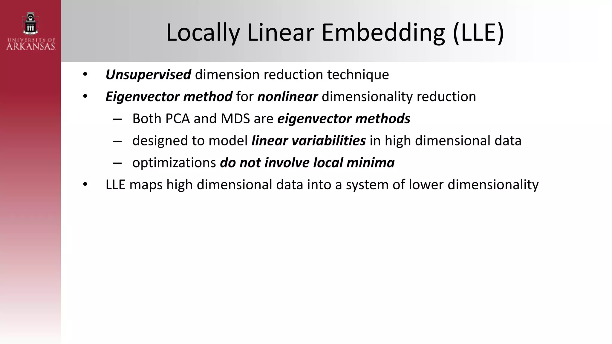
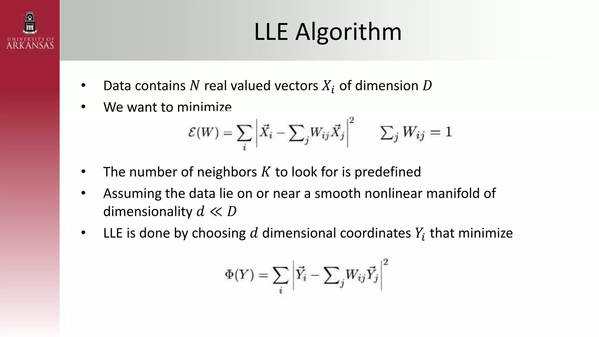
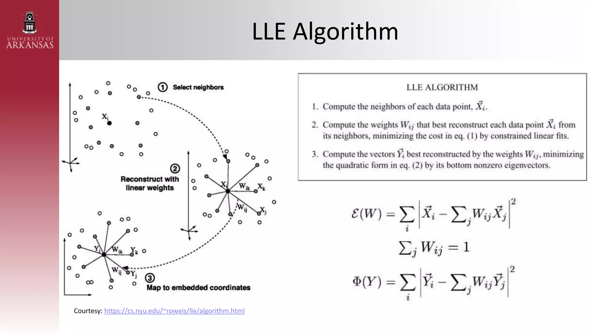
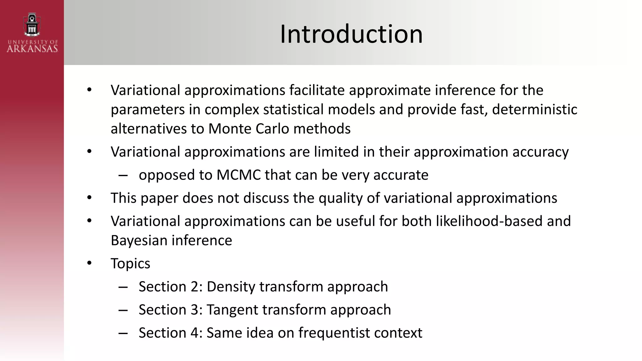
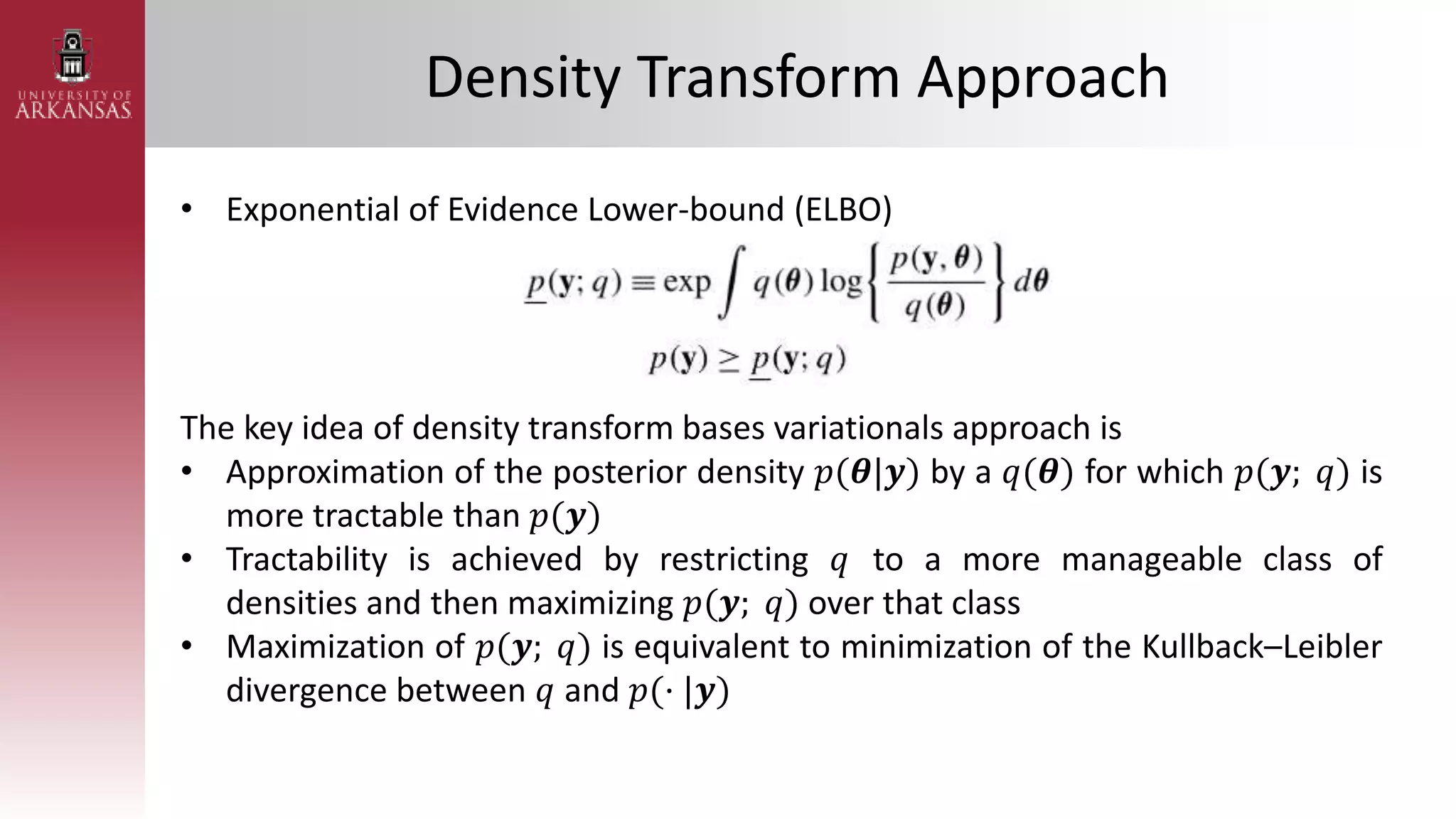
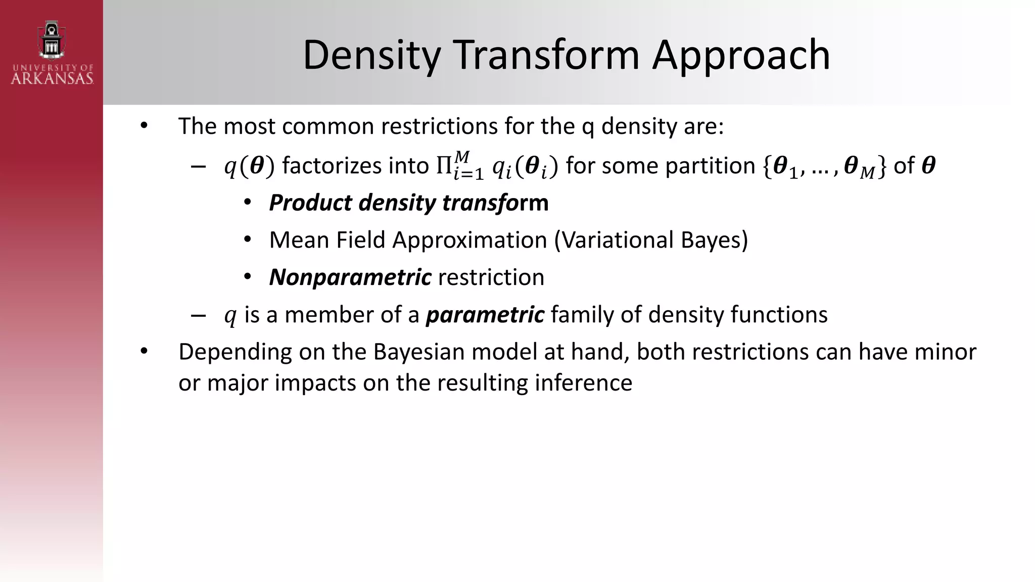
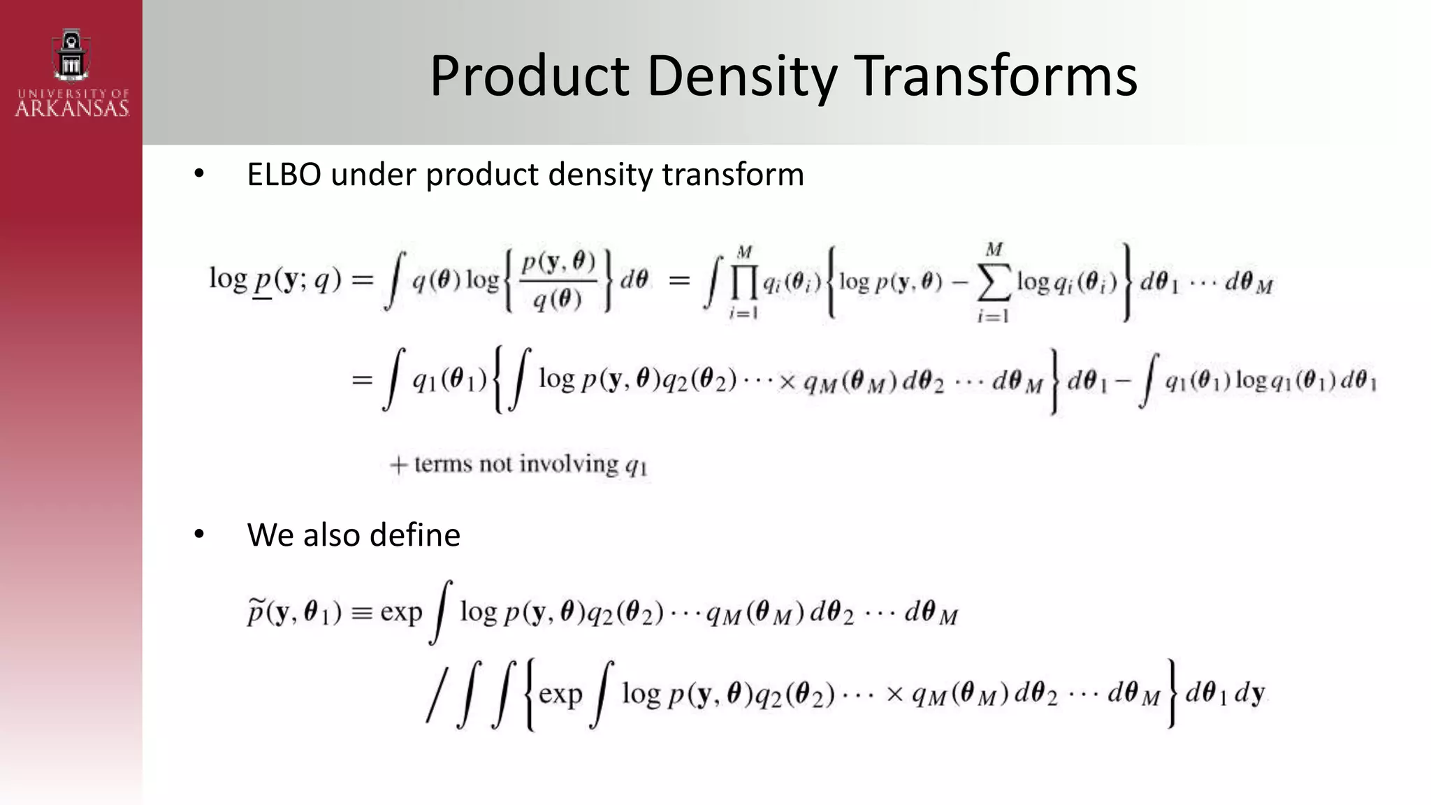
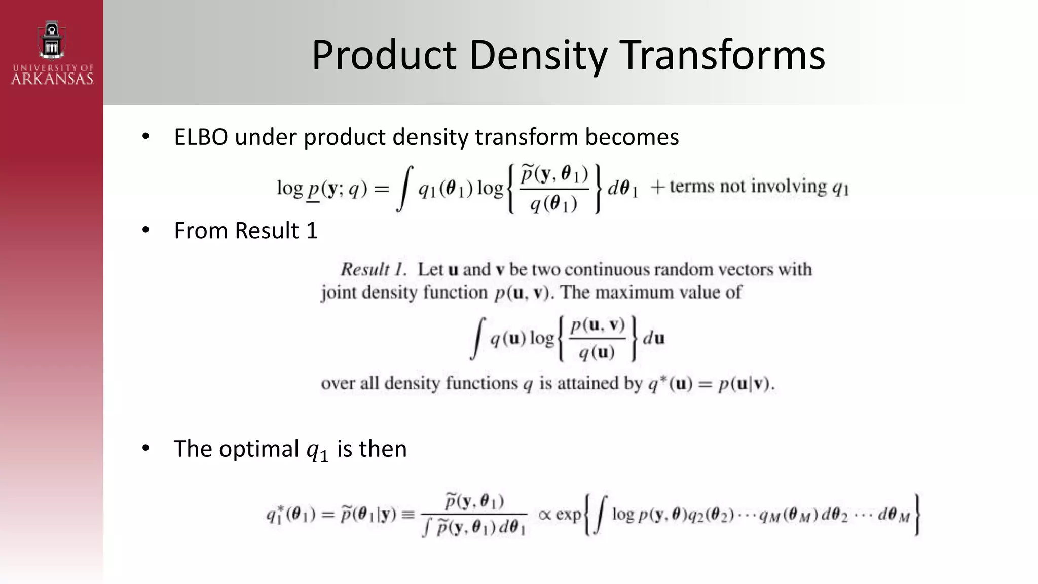
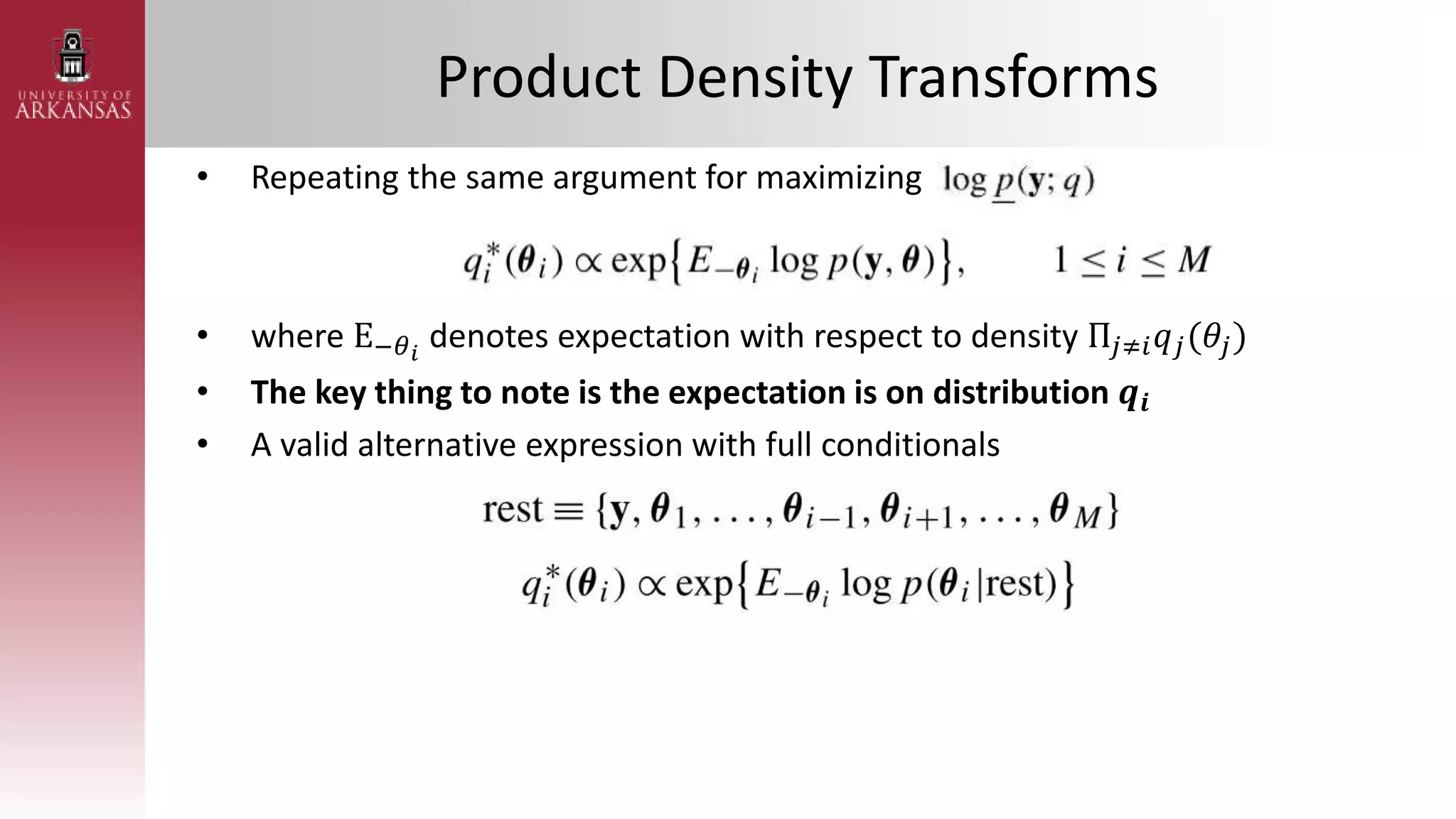
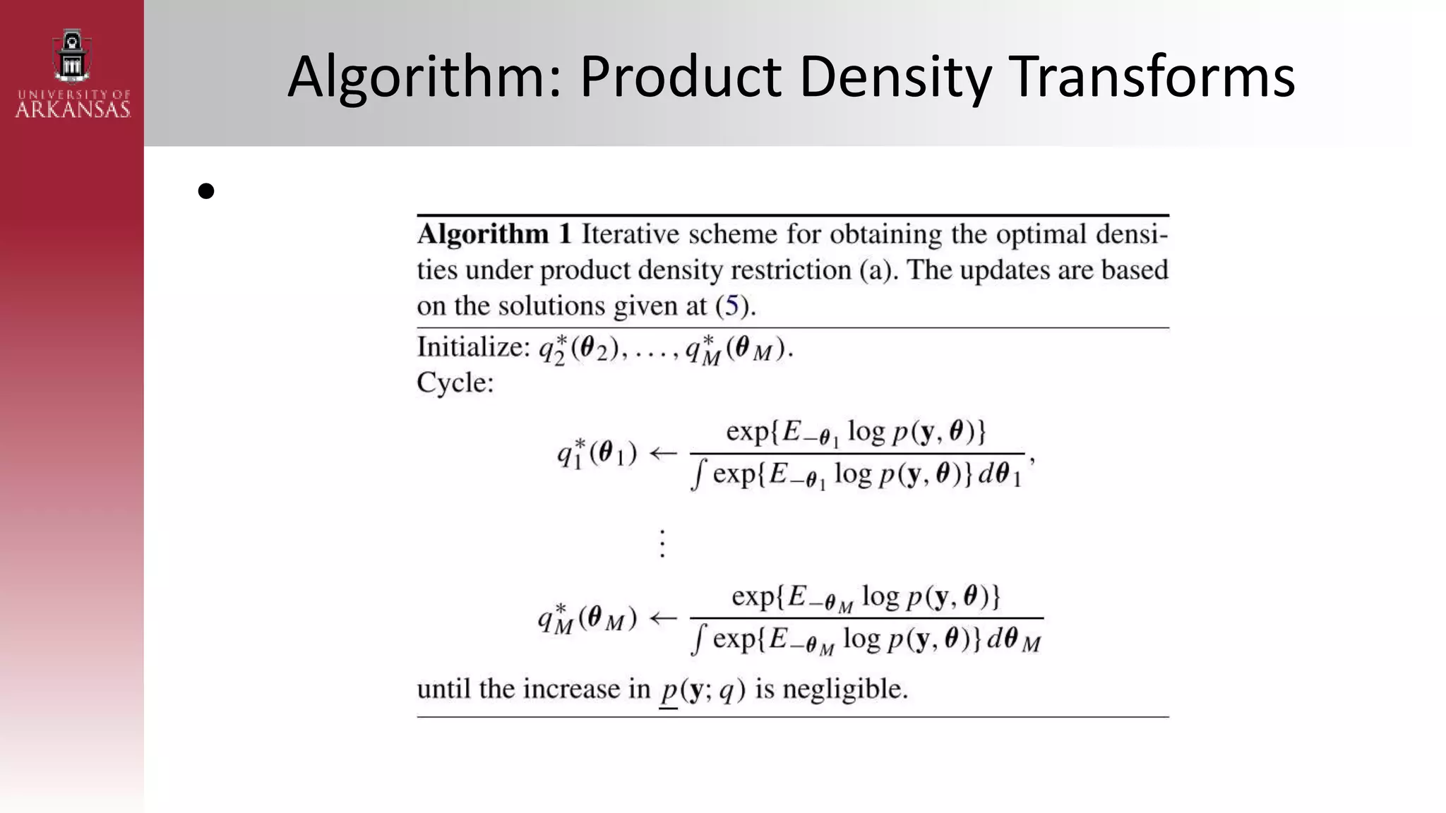
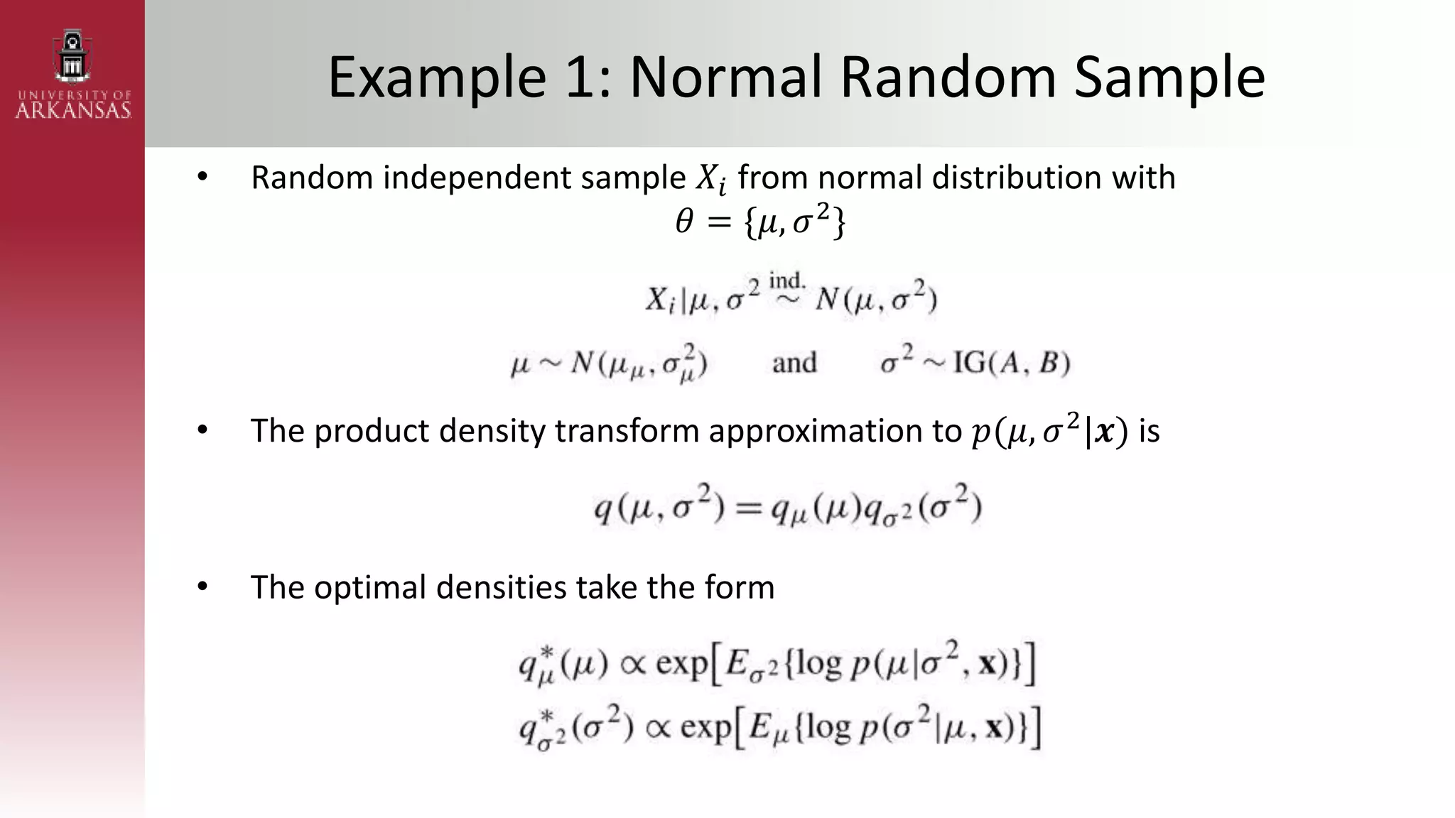
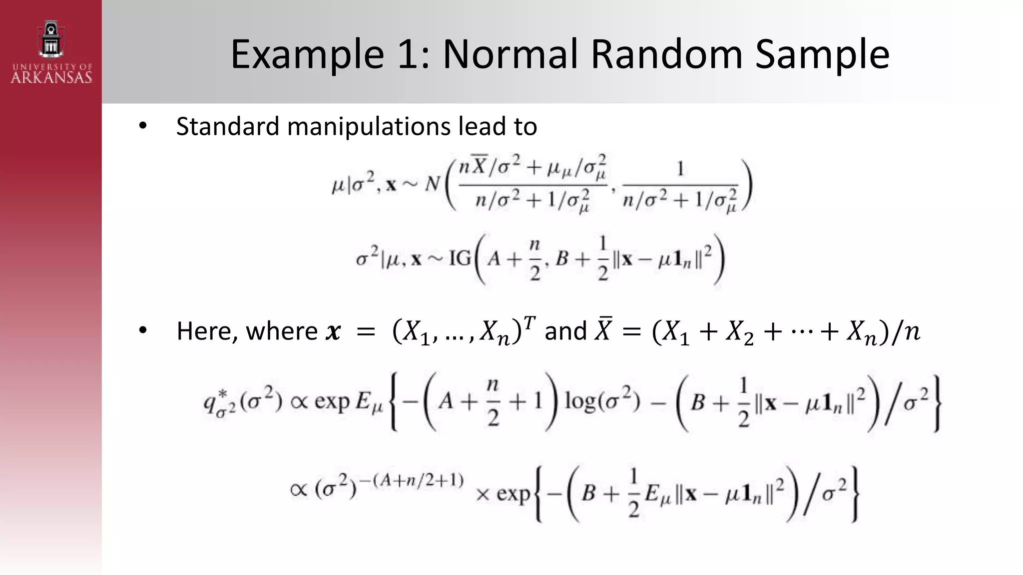
This document provides a summary of three topics: 1) An introduction to Locally Linear Embedding (LLE), an unsupervised nonlinear dimensionality reduction technique. It describes the objective, idea, and algorithm of LLE. 2) Explaining variational approximations, describing the idea, algorithm, and examples of both density transform and tangent transform approaches. Variational approximations provide fast deterministic alternatives to Monte Carlo methods. 3) A question and answer section.

1. Comprehensive Examination
Master’s in Statistics and Analytics
Md Abul Hayat
Graduate Assistant
Electrical Engineering
April 26, 2021

2. Contents
• An Introduction to Locally Linear Embedding
– Objective
– Idea
– Algorithm
– Results
• Explaining Variational Approximations
– Idea
– Algorithm
– Examples
• Q&A

3. An Introduction to Locally Linear Embedding
Lawrence K. Saul, Sam T. Roweis
Unpublished (2000)
Available at https://cs.nyu.edu/~roweis/lle/publications.html

4. Locally Linear Embedding (LLE)
• Unsupervised dimension reduction technique
• Eigenvector method for nonlinear dimensionality reduction
– Both PCA and MDS are eigenvector methods
– designed to model linear variabilities in high dimensional data
– optimizations do not involve local minima
• LLE maps high dimensional data into a system of lower dimensionality

5. LLE Algorithm
• Data contains 𝑁 real valued vectors 𝑋𝑖 of dimension 𝐷
• We want to minimize
• The number of neighbors 𝐾 to look for is predefined
• Assuming the data lie on or near a smooth nonlinear manifold of
dimensionality 𝑑 ≪ 𝐷
• LLE is done by choosing 𝑑 dimensional coordinates 𝑌𝑖 that minimize

6. LLE Algorithm
Courtesy: https://cs.nyu.edu/~roweis/lle/algorithm.html

7. Constrained Least Squares Problem
• Step 1:
s.t.
• Notations
• Cost Function

8. Constrained Least Squares Problem
• Cost Function
• Assuming,
• The cost function becomes
• Optimization

9. Eigenvector Problem
• Step-2
• Notation
– 𝑊𝑖 is i-th column of 𝑛 𝑥 𝑛 weight matrix 𝑊
– 𝐼𝑖 is i-th column of 𝑛 𝑥 𝑛 identity matrix 𝐼
• Using this notation

10. Eigenvector Problem
• This gives
• Replacing 𝑀
• The solution 𝑌 consists of 𝑑 eigenvectors of 𝑀 corresponding to 2 to 𝑑 + 1
minimum eigenvalues

11. Results

12. Results

13. Explaining Variational Approximations
John T. Ormerod, Matt P. Wand
The American Statistician (2010)

14. Introduction
• Variational approximations facilitate approximate inference for the
parameters in complex statistical models and provide fast, deterministic
alternatives to Monte Carlo methods
• Variational approximations are limited in their approximation accuracy
– opposed to MCMC that can be very accurate
• This paper does not discuss the quality of variational approximations
• Variational approximations can be useful for both likelihood-based and
Bayesian inference
• Topics
– Section 2: Density transform approach
– Section 3: Tangent transform approach
– Section 4: Same idea on frequentist context

15. Density Transform Approach
• Consider a generic Bayesian model with parameter vector 𝜃 ∈ Θ and
observed data vector 𝒚
• Posterior density function
• The denominator 𝑝(𝒚) is known as the marginal likelihood
– model evidence in the Computer Science literature
• Assuming q to be an arbitrary density function and q ∈ Θ

16. Density Transform Approach
equality if and only if 𝑞(𝜽) = 𝑝(𝜽|𝒚)

17. Density Transform Approach
• Exponential of Evidence Lower-bound (ELBO)
The key idea of density transform bases variationals approach is
• Approximation of the posterior density 𝑝(𝜽|𝒚) by a 𝑞(𝜽) for which 𝑝(𝒚; 𝑞) is
more tractable than 𝑝(𝒚)
• Tractability is achieved by restricting 𝑞 to a more manageable class of
densities and then maximizing 𝑝(𝒚; 𝑞) over that class
• Maximization of 𝑝(𝒚; 𝑞) is equivalent to minimization of the Kullback–Leibler
divergence between 𝑞 and 𝑝(· |𝒚)

18. Density Transform Approach
• The most common restrictions for the q density are:
– 𝑞(𝜽) factorizes into Π𝑖=1
𝑀
𝑞𝑖(𝜽𝑖) for some partition {𝜽1, … , 𝜽𝑀} of 𝜽
• Product density transform
• Mean Field Approximation (Variational Bayes)
• Nonparametric restriction
– 𝑞 is a member of a parametric family of density functions
• Depending on the Bayesian model at hand, both restrictions can have minor
or major impacts on the resulting inference

19. Product Density Transforms
• ELBO under product density transform
• We also define

20. Product Density Transforms
• ELBO under product density transform becomes
• From Result 1
• The optimal 𝑞1 is then

21. Product Density Transforms
• Repeating the same argument for maximizing
• where E−𝜃𝑖
denotes expectation with respect to density Π𝑗≠𝑖𝑞𝑗(𝜃𝑗)
• The key thing to note is the expectation is on distribution 𝒒𝒊
• A valid alternative expression with full conditionals

22. Algorithm: Product Density Transforms
•

23. Example 1: Normal Random Sample
• Random independent sample 𝑋𝑖 from normal distribution with
𝜃 = {𝜇, 𝜎2
}
• The product density transform approximation to 𝑝(𝜇, 𝜎2
|𝒙) is
• The optimal densities take the form

24. Example 1: Normal Random Sample
• Standard manipulations lead to
• Here, where 𝒙 = 𝑋1, … , 𝑋𝑛
𝑇
and 𝑋 = (𝑋1 + 𝑋2 + ⋯ + 𝑋𝑛)/𝑛

25. Example 1: Normal Random Sample
• Optimal densities
• Also
• ELBO

26. Example 1: Normal Random Sample
• Algorithm and result

27. Example 2: Linear Mixed Model
• Bayesian Gaussian Linear Mixed Model
– 𝒀 and 𝜷 are a 𝑛𝑥1 and 𝑝𝑥1 vector respectively
– Variance component model
– Conjugate priors

28. Example 2: Linear Mixed Model
• Tractable solution arises for two component model
• Let 𝝁𝑞 𝜷, 𝒖 and Σ𝑞(𝜷, 𝒖) be the mean and covariance of 𝑞∗ 𝜷, 𝒖
• Set 𝑪 = 𝑿 𝒁
• Markov blanket

29. Example 2: Linear Mixed Model
•
• Upon convergence the approximate posteriors are:

30. Example 2: Linear Mixed Model
• Longitudinal Orthodontic Measurement (Pinherio and Bates 2000)
• Model
• Comparing with
• Here

31. Example 2: Linear Mixed Model
•

32. Example 3: Probit Regression
• Bayesian probit regression
• Likelihood
• Auxiliary variable

33. Example 3: Probit Regression
• Product density

34. Example 4: Finite Mixture Model
• Let (𝑋1, 𝑋2, ⋯ 𝑋𝑛) be univariate samples that are modeled as mixture of 𝐾
normal density functions with parameter (𝜇𝑘, 𝜎𝑘
2
)
• Auxiliary variable

35. Example 4: Finite Mixture Model
•
•

36. Parametric Density Transform
• Poisson Regression with Gaussian Transform
– Assuming 𝜷 ∼ (𝝁𝜷, 𝚺𝜷) and 𝑿 = [1 𝑥1𝑖 ⋯ 𝑥𝑘𝑖]
• Likelihood
• Marginal likelihood
• Take the 𝑞 𝛽 = 𝑁(𝝁𝑞 𝛽 , 𝚺𝑞(𝛽)) density

37. Tangent Transform Approach
• Work with ‘tangent-type’ representations of concave and convex functions
– The value of 𝜉 can then be chosen to make the approximation as accurate as possible.

38. Bayesian Logistic Regression
• Model
• Likelihood
• Assuming 𝜷 ∼ 𝝁𝜷, 𝚺𝜷 , the posterior of 𝜷 is
– Here

39. Bayesian Logistic Regression
• Here
• Similarly
• Lower bound on 𝑝(𝒚, 𝜷)

40. Bayesian Logistic Regression
• Maximizing the following term using EM gives us the solution

41. Questions?

42. Thanks for listening :D