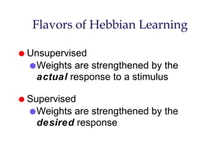
The document discusses various types of Hebbian learning including: 1) Unsupervised Hebbian learning where weights are strengthened based on actual neural responses to stimuli without a target output. 2) Supervised Hebbian learning where weights are strengthened based on the desired neural response rather than the actual response to better approximate a target output. 3) Recognition networks like the instar rule which only updates weights when a neuron's output is active to recognize specific input patterns.

1. Next Assignment Train a counter-propagation network to compute the 7-segment coder and its inverse. You may use the code in /cs/cs152/book: counter.c readme

2. ART1 Demo Increasing vigilance causes the network to be more selective, to introduce a new prototype when the fit is not good. Try different patterns

3. Hebbian Learning

4. Hebb’s Postulate “ When an axon of cell A is near enough to excite a cell B and repeatedly or persistently takes part in firing it, some growth process or metabolic change takes place in one or both cells such that A’s efficiency, as one of the cells firing B, is increased.” D. O. Hebb, 1949 A B In other words, when a weight contributes to firing a neuron, the weight is increased. (If the neuron doesn’t fire, then it is not).

5. A B

6. A B

7. Colloquial Corollaries “ Use it or lose it”.

8. Colloquial Corollaries? “ Absence makes the heart grow fonder”.

9. Generalized Hebb Rule When a weight contributes to firing a neuron, the weight is increased. When a weight acts to inhibit the firing of a neuron, the weight is decreased .

10. Flavors of Hebbian Learning Unsupervised Weights are strengthened by the actual response to a stimulus Supervised Weights are strengthened by the desired response

11. Unsupervised Hebbian Learning (aka Associative Learning)

12. Simple Associative Network input output

13. Banana Associator Unconditioned Stimulus Conditioned Stimulus Didn’t Pavlov anticipate this?

14. Banana Associator Demo can be toggled

15. Unsupervised Hebb Rule Vector Form: Training Sequence: actual response input

16. Learning Banana Smell Initial Weights: Training Sequence: First Iteration (sight fails, smell present):  = 1 unconditioned (shape) conditioned (smell) a 1   h a r d l i m w 0 p 0 1   w 0   p 1   0.5 – +   h a r d l i m 1 0  0 1  0.5 – +   0 (no banana) = = =

17. Example Second Iteration (sight works, smell present): Third Iteration (sight fails, smell present): Banana will now be detected if either sensor works. a 2   h a r d l i m w 0 p 0 2   w 1   p 2   0.5 – +   h a r d l i m 1 1  0 1  0.5 – +   1 (banana) = = =

18. Problems with Hebb Rule Weights can become arbitrarily large. There is no mechanism for weights to decrease.

19. Hebb Rule with Decay This keeps the weight matrix from growing without bound, which can be demonstrated by setting both a i and p j to 1:

20. Banana Associator with Decay

21. Example: Banana Associator First Iteration (sight fails, smell present): Second Iteration (sight works, smell present):  = 0.1  = 1 a 1   h a r d l i m w 0 p 0 1   w 0   p 1   0.5 – +   h a r d l i m 1 0  0 1  0.5 – +   0 (no banana) = = = a 2   h a r d l i m w 0 p 0 2   w 1   p 2   0.5 – +   h a r d l i m 1 1  0 1  0.5 – +   1 (banana) = = =

22. Example Third Iteration (sight fails, smell present):

23. General Decay Demo no decay larger decay w i j m a x   - - - =

24. Problem of Hebb with Decay Associations will be lost if stimuli are not occasionally presented. If a i = 0, then If  = 0, this becomes Therefore the weight decays by 10% at each iteration where there is no stimulus.

25. Solution to Hebb Decay Problem Don’t decay weights when there is no stimulus We have seen rules like this (Instar)

26. Instar (Recognition Network)

27. Instar Operation The instar will be active when or For normalized vectors, the largest inner product occurs when the angle between the weight vector and the input vector is zero -- the input vector is equal to the weight vector. The rows of a weight matrix represent patterns to be recognized. w T 1 p w 1 p  cos b –  =

28. Vector Recognition If we set the instar will only be active when   =  0. If we set the instar will be active for a range of angles. As b is increased, the more patterns there will be (over a wider range of  ) which will activate the instar. b w 1 p – = b w 1 p – > w 1

29. Instar Rule Hebb with Decay Modify so that learning and forgetting will only occur when the neuron is active - Instar Rule: or Vector Form: w i j q   w i j q 1 –    a i q   p j q    a i q   w q 1 –   – + = i j

30. Graphical Representation For the case where the instar is active ( a i = 1): or For the case where the instar is inactive ( a i = 0):

31. Instar Demo weight vector input vector  W

32. Outstar ( Recall Network)

33. Outstar Operation Suppose we want the outstar to recall a certain pattern a * whenever the input p = 1 is presented to the network. Let Then, when p = 1 and the pattern is correctly recalled. The columns of a weight matrix represent patterns to be recalled.

34. Outstar Rule For the instar rule we made the weight decay term of the Hebb rule proportional to the output of the network. For the outstar rule we make the weight decay term proportional to the input of the network. If we make the decay rate  equal to the learning rate  , Vector Form:

35. Example - Pineapple Recall

36. Definitions

37. Outstar Demo

38. Iteration 1  = 1

39. Convergence

40. Supervised Hebbian Learning

41. Linear Associator Training Set:

42. Hebb Rule Presynaptic Signal Postsynaptic Signal Simplified Form: Supervised Form: Matrix Form: actual output input pattern desired output

43. Batch Operation Matrix Form: (Zero Initial Weights)  W t 1 t 2  t Q p 1 T p 2 T p Q T T P T = = T t 1 t 2  t Q = P p 1 p 2  p Q =

44. Performance Analysis Case I, input patterns are orthogonal. Therefore the network output equals the target: Case II, input patterns are normalized, but not orthogonal. Error term 0 q k  =

45. Example Banana Apple Normalized Prototype Patterns Weight Matrix (Hebb Rule): Tests: Banana Apple

46. Pseudoinverse Rule - (1) Performance Index: Matrix Form: Mean-squared error T t 1 t 2  t Q = P p 1 p 2  p Q = || E || 2 e i j 2 j  i  =

47. Pseudoinverse Rule - (2) Minimize: If an inverse exists for P , F ( W ) can be made zero: When an inverse does not exist F ( W ) can be minimized using the pseudoinverse:

48. Relationship to the Hebb Rule Hebb Rule Pseudoinverse Rule If the prototype patterns are orthonormal: W T P T =

49. Example

50. Autoassociative Memory

51. Tests 50% Occluded 67% Occluded Noisy Patterns (7 pixels)

52. Supervised Hebbian Demo

53. Spectrum of Hebbian Learning Basic Supervised Rule: Supervised with Learning Rate: Smoothing: Delta Rule: Unsupervised: target actual